1506
Improved MR thermometry for laser-induced thermal therapy – tradeoffs between imaging approaches1Radiology and Imaging Sciences, University of Utah, Salt Lake City, UT, United States
Synopsis
MR thermometry is often used to monitor thermal therapies such as focused ultrasound and laser induced thermal therapies (LITT). As in MRI in general, there is an inherent tradeoff between measurement accuracy, precision, and spatial and temporal resolution in MR thermometry. In this work we present improved acquisition protocols for 2D and 3D MR thermometry for LITT applications. We investigate and compare image quality and temperature precision for 8 different 2D and 3D GRE, and 3D segmented EPI protocols. Experiments are performed in a healthy volunteer (non-heating) and tissue-mimicking gel (with heating).
Introduction
MRI has become the image modality of choice to monitor many non- and minimally-invasive interventional procedures such as focused ultrasound and laser-inducer thermal therapy (LITT) because it combines high-resolution anatomical imaging for procedure guidance with real-time MR temperature imaging (MRTI) for procedure monitoring. The proton resonance frequency shift (PRFS) method (1,2) is the most commonly used MRTI approach as it has been shown to work for a wide range of (aqueous) tissues and is linear over a relatively large temperature range (3). As in MR in general, there are some inherent trade-offs between field of view, spatial resolution, temporal resolution, and measurement precision in MRTI. In this work we compare different 2D and 3D approaches for performing MRTI for LITT applications in the brain using the PRFS approach. We investigate trade-offs in MRTI precision, image quality (distortion) and off-resonance effects for 2D and 3D gradient recalled echo (GRE), and 3D echo-planar imaging (EPI) approaches.Methods
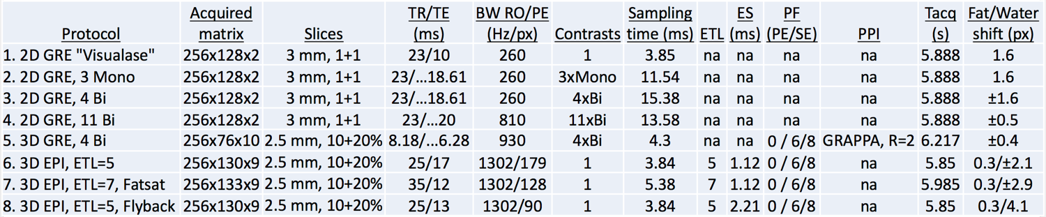
Table 1 lists the 8 protocol approaches investigated in this work. #1 is the 2DGRE protocol currently used clinically with our LITT system (Visualase™ MRI-Guided Laser Ablation System, Louisville, CO), where 2 orthogonal 2D slices (usually oriented along the laser fiber in Sagittal+Coronal planes) are being sampled. Using the same TR and BW (23 ms, 260 Hz/px), 3 mono- or 4 bi-polar contrasts can be acquired (#2-#3) on our scanner (80mT/m gradient, 200T/m/s slew rates). This increases the total sampling time from 3.85ms to 11.54 and 15.38ms, respectively, improving MRTI precision by sqrt(sampling time) (1.7-2.0x) with no scan time penalty. #4 is 2DGRE with increased BW (810Hz/px) to reduce off-resonance shift from temperature change/fat. #5 is 3DGRE acquiring 12 slices in the same scan time as the 2DGRE protocols. #6-#8 are 3D segmented-EPI with mono- (i.e., flyback) and bi-polar readouts and varying ETL to investigate differences in off-resonance effects and distortion.
Scans were performed on a 3T scanner (PrismaFIT, Siemens, Erlangen, Germany) with a 4-channel wrap-around/flex-coil. In-vivo scans were performed on one healthy volunteer under IRB-approved informed consent. LITT sonications were performed in a human-sized plastic skull (3B Scientific, Tucker, GA) filled with tissue-mimicking gellan gum (Fisher Scientific, Pittsburgh, PA) at 3W for 8 dynamic measurements (~47-50 s), and were repeated 3 times/protocol. All data was zero-filled interpolated (for 2D only in-plane, and for 3D in all 3 directions) to 0.5-mm voxel spacing to minimize partial volume effects. MRTI utilized referenceless reconstruction (4). Measured T1 (in vivo/phantom ~1000/~1800 ms) was used to calculate and apply the Ernst angle for all protocols.
Results
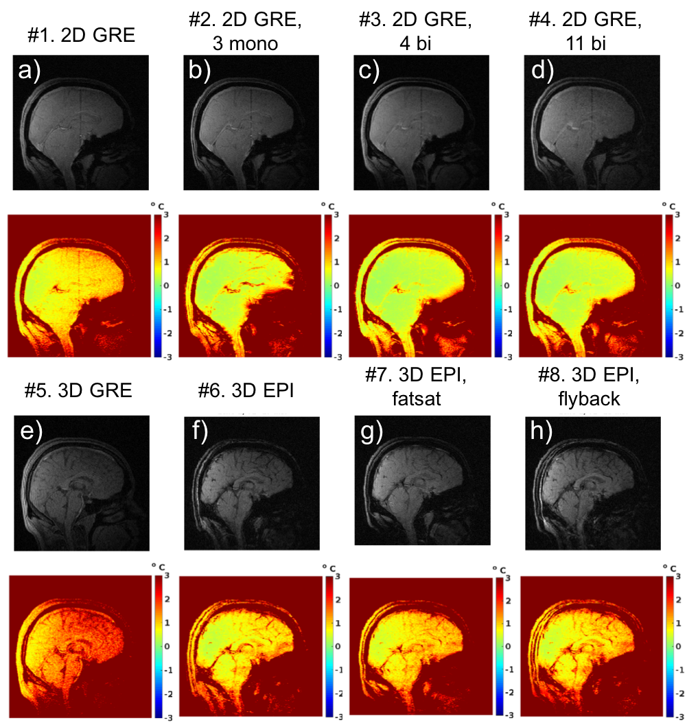
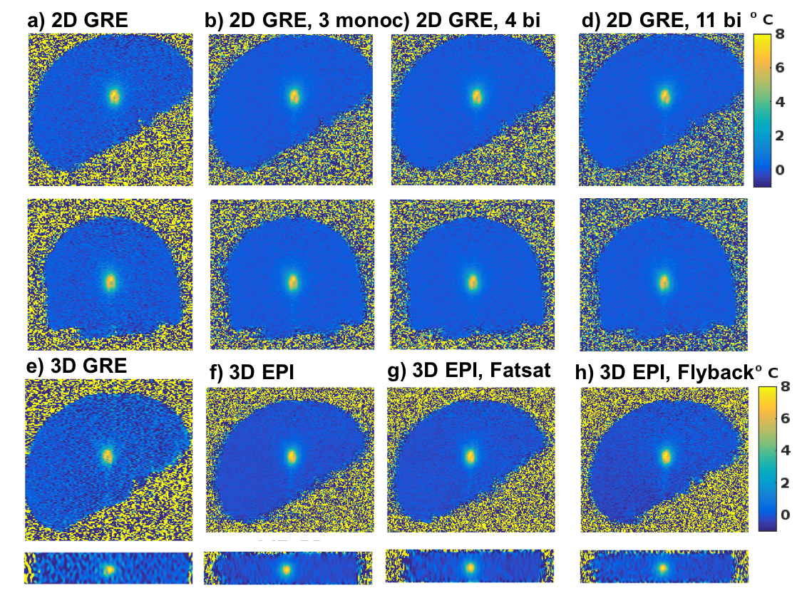
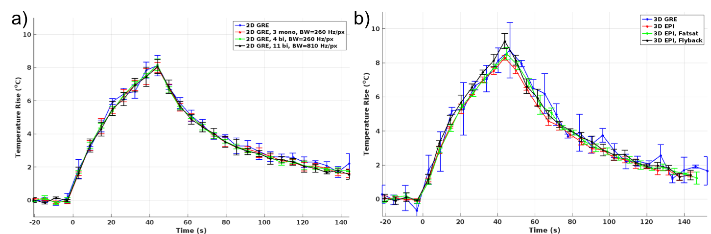
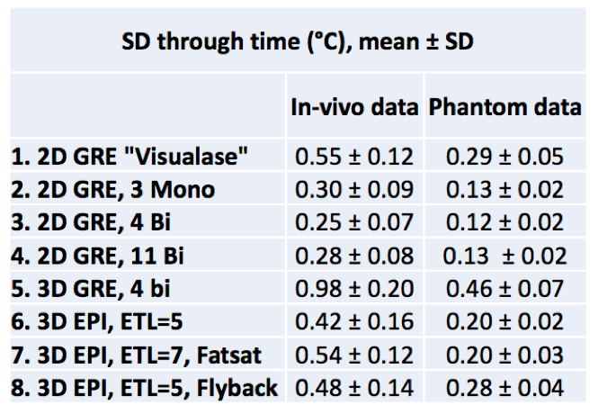
Figure 1 shows magnitude and temperature standard deviation (SD) through time maps from a central sagittal slice in the volunteer for all 8 protocols. Figure 2 shows two orthogonal views of temperature maps at time of maximum heating, and Figure 3 shows temperature vs. time plots for the hottest voxel (mean±SD of three heatings), both for the phantom experiment. Table 2 lists the precision of the measurements, defined as the SD through time of an (un-heated) background region.Discussion and Conclusions
Table 2 shows that the best MRTI precision was achieved with multi-contrast 2D protocols, followed by 3DEPI, single-contrast 2DGRE, and last 3DGRE. This agrees well with theory and sampling time duration for the different protocols (Table 1). The precision of 3DGRE is negatively affected by the parallel imaging (resulting in at least sqrt(R) SNR decrease), needed to achieve similar scan time. The higher maximum temperature rise measured in 3D protocols compared to 2D protocols (Figure 3) is likely due to reduced partial-volume effects due to the ZFI in three-dimensions vs only two-dimensions for 2D protocols. All 2D protocols show good SNR magnitude images with minimal distortions. The high-BW protocol (#4) shows the least fat-water shift (~1 voxel) and the 4 contrast bi-polar protocol (#3) show the largest shift (~3 voxels) – seen comparing the skin-fat layer around the skull (RO direction is H->F for sagittal images). 3D protocols all have high RO-BW and experience the smallest fat-water shift (all <1 voxel), but EPI sequences have rather low PE-BW and experience larger shifts in this direction (A->P). This is most clearly seen in the flyback protocol which has the lowest PE-BW.
To maximize MRTI precision, the available TR should be filled with multiple contrasts. The already high RO-BW allows for bi-polar readout without large off-resonance shifts. 3D EPI imaging with good precision, albeit somewhat more distortions, can be achieved in the same scan time. 3D GRE achieves small distortions, but for similar precision scan time increases are needed.
Acknowledgements
This work was supported by Medtronic and the Mark H. Huntsman endowed chair.References
1. De Poorter J. Noninvasive MRI thermometry with the proton resonance frequency method Study of susceptibility effects. Magn. Reson. Med. 1995;43:359–67.
2. Ishihara Y, Calderon A, Watanabe H, Okamoto K, Suzuki Y, Kuroda K. A precise and fast temperature mapping using water proton chemical shift. Magn. Reson. Med. 1995;34:814–23.
3. Rieke V, Butts Pauly K. MR thermometry. J. Magn. Reson. Imaging 2008;27:376–90. doi: 10.1002/jmri.21265.
4. Rieke V, Vigen KK, Sommer G, Daniel BL, Pauly JM, Butts K. Referenceless PRF shift thermometry. Magn. Reson. Med. 2004;51:1223–1231. doi: 10.1002/mrm.20090.
Figures