1486
Temperature Induced Susceptibility Correlation in Adipose Tissues for MR-Guided Microwave Ablation1Department of Biomedical Engineering, Tsinghua University, Beijing, China, 2Department of Engineering Physics, Tsinghua University, Beijing, China, 3Department of Orthopedics, First Affiliated Hospital of PLA General Hospital, Beijing, China, 4Key Laboratory of Particle and Radiation Imaging, Ministry of Education, Medical Physics and Engineering Institute, Tsinghua University, Beijing, China
Synopsis
Microwave ablation requires high temperature measurement accuracy to monitor the curative effect of the lesions. PRFS-based MR thermometry is the most commonly used temperature monitoring technique. However, PRFS is hampered by temperature-dependent magnetic susceptibility changes. It has been proved in the Quantitative Susceptibility Mapping(QSM) that susceptibility can be measured from the phase changes ,which is derived from Maxwell’s Equation. In this work, we proposed a practical method to calculate the errors caused by temperature-induced susceptibility changes based on the method in QSM. Both Simulation studies and microwave heating experiments validated the accuracy of the method.
Purpose
In microwave ablation, it is important to achieve accurate real-time temperature monitoring for operations. Considering the poor performance of PRF-method, many methods have been proposed which could effectively improve the accuracy. However, in tissues containing fat, temperature-induced susceptibility changes in fat may greatly disturb the magnetic field in the surroundings sites and lead to large errors in temperature estimation.1 As temperature induced susceptibility changes in fat is much larger than that in water, an algorithm is proposed in Quantitative Susceptibility Mapping (QSM) based on Maxwell’s Equation to calculate the underlying susceptibility distribution from the phase data.2,3 In this work, we proposed a practical method to calculate the errors caused by temperature-induced susceptibility changes based on the method from QSM for its accuracy.Methods
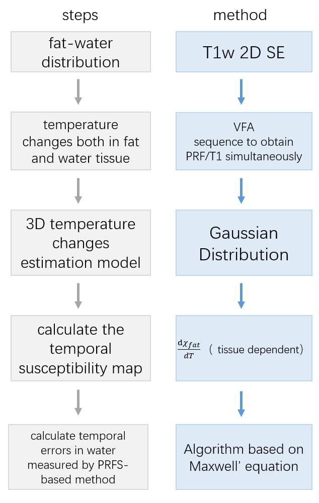
The main steps of the proposed method to correct the susceptibility error are shown in Fig.1.
Variable Flip Angle was utilized to simutaneously acquire temperature data in water and fat tissues. In principle, the disturbance caused by temperature-induced magnetic field changes in fat occurs in the whole heated volume. To reach high temporal resolution during thermal ablation, 3D temperature changes in heated areas is estimated by a Gaussian distribution model to estimate the 3D temperature-induced susceptibility changes. The measured PRFS temperature change in water can be calculated by adding the contribution from temperature-induced susceptibility changes, which is calculated as:
$$\Delta \phi _{sus} = (2\pi \gamma B_0 T_E )F^{-1}DF(\chi _{fat} + \frac{d\chi_{fat}}{dT}) - (2\pi \gamma B_0 T_E )F^{-1}DF(\chi _{fat})$$
$$ \Delta \phi_{real} = \Delta \phi_{PRF} + \Delta \phi _{sus} $$
$$\Delta T_{real} = \frac{\Delta \phi_{real}}{\gamma \alpha B_0 T_E}$$
where $$$\gamma$$$ is magnetogyric ratio, $$$D=(\frac{1}{3}-cos^2\beta)$$$ represents the Fourier transform of the convolution kernel that links the susceptibility and field, $$$chi$$$ the susceptibility, B0 the magnetic field strength, TE the echo time, $$$\alpha$$$ the thermal coefficient($$$\alpha=0.01ppm ^\circ C$$$) , $$$\Delta \phi _{sus} $$$ the temperature errors caused by susceptibility changes.
Experimental Designs
The phantom experiments with heating simulation were performed to investiage the accuracy of the our proposed method, and the data were acquired on a 3.0T Philips system (Philips Healthcare, Best, the Netherland) and in-plane resolution of all experiment is 2×2 mm2 .
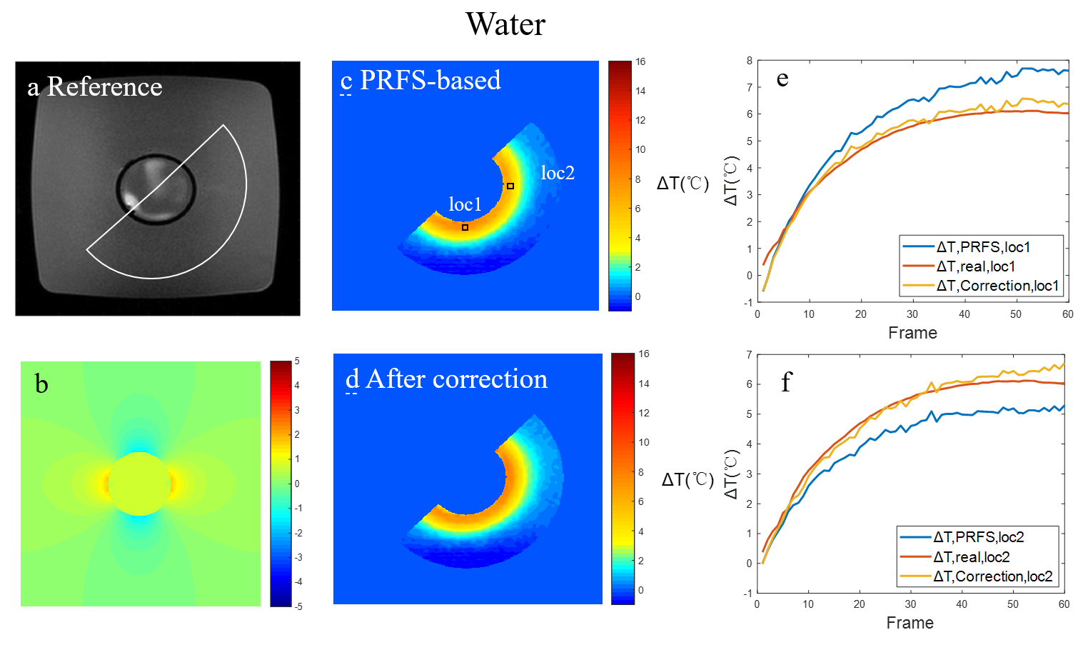
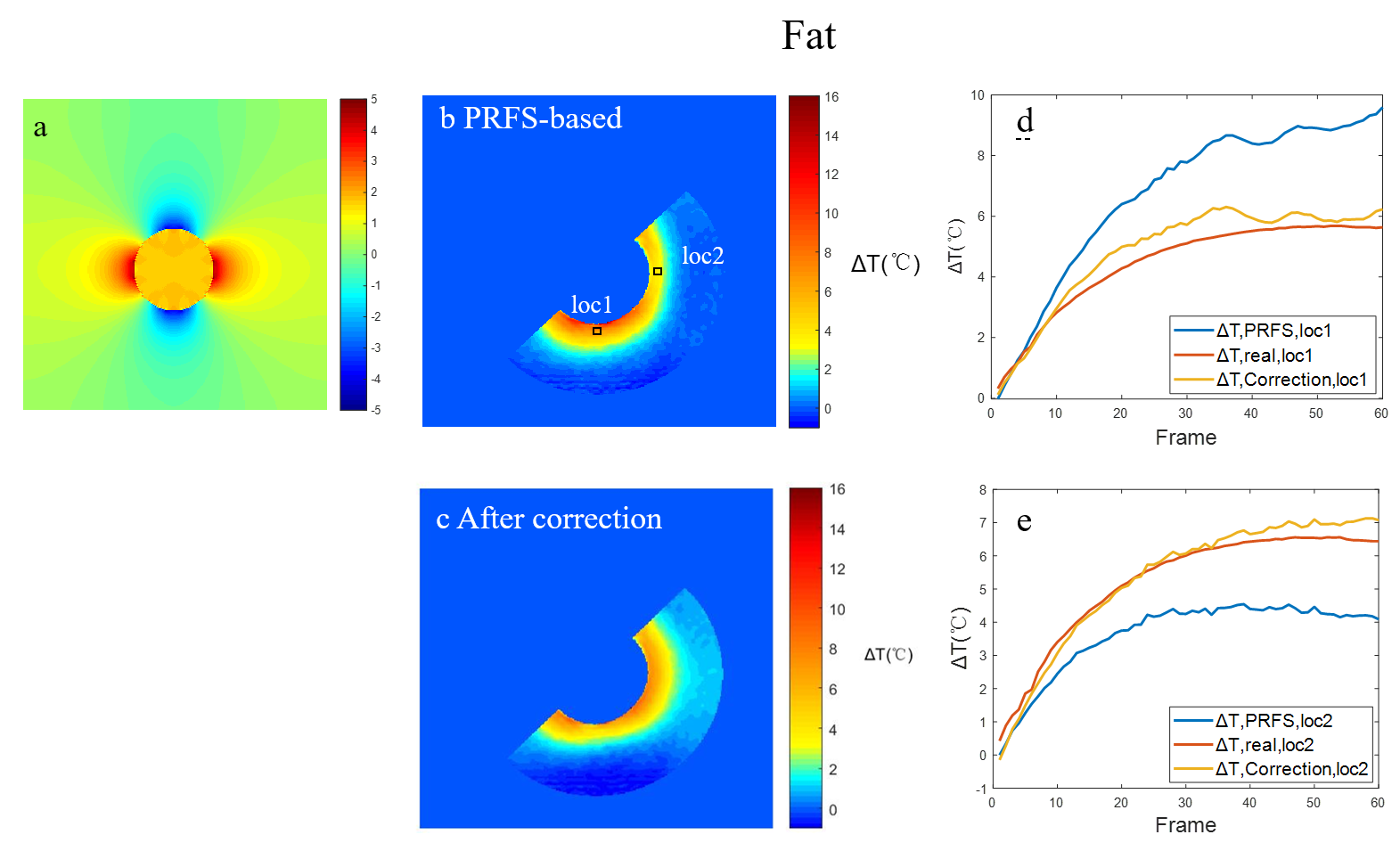
Two phantom cooling experiments were conducted to validate the proposed correction algorithm. The phantom consisted of a rectangular water gel (150×150×60mm3, 1% agar) with a Perspex cylinder (outer radius = 22.5mm; inner radius = 20.5mm; length = 80mm) placed in the center, which contained liquid water and sunflower oil. The liquid in the center was heated to 60$$$^\circ C$$$ by water bath and cooling down during scanning. The 2D T1w GRE sequence was implemented. The scan parameters were: FOV = 160×160 mm2,TR/TE = 50/15 ms, flip angle = 30°, dynamic scan time = 9sec.
A lard oil cooling experiment was conducted to determine the temperature dependence of extracted lard oil. The lard oil was heated to 60$$$^\circ C$$$ by water bath and cooling down to 43.5$$$^\circ C$$$ during scanning. The Variable Flip Angle(VFA) sequence with three different flip angle was implemented. The scan parameters were: FOV = 160×160 mm2,TR/TE = 9/2.4 ms, flip angle = 4°/10°/20°, dynamic scan time = 5sec.
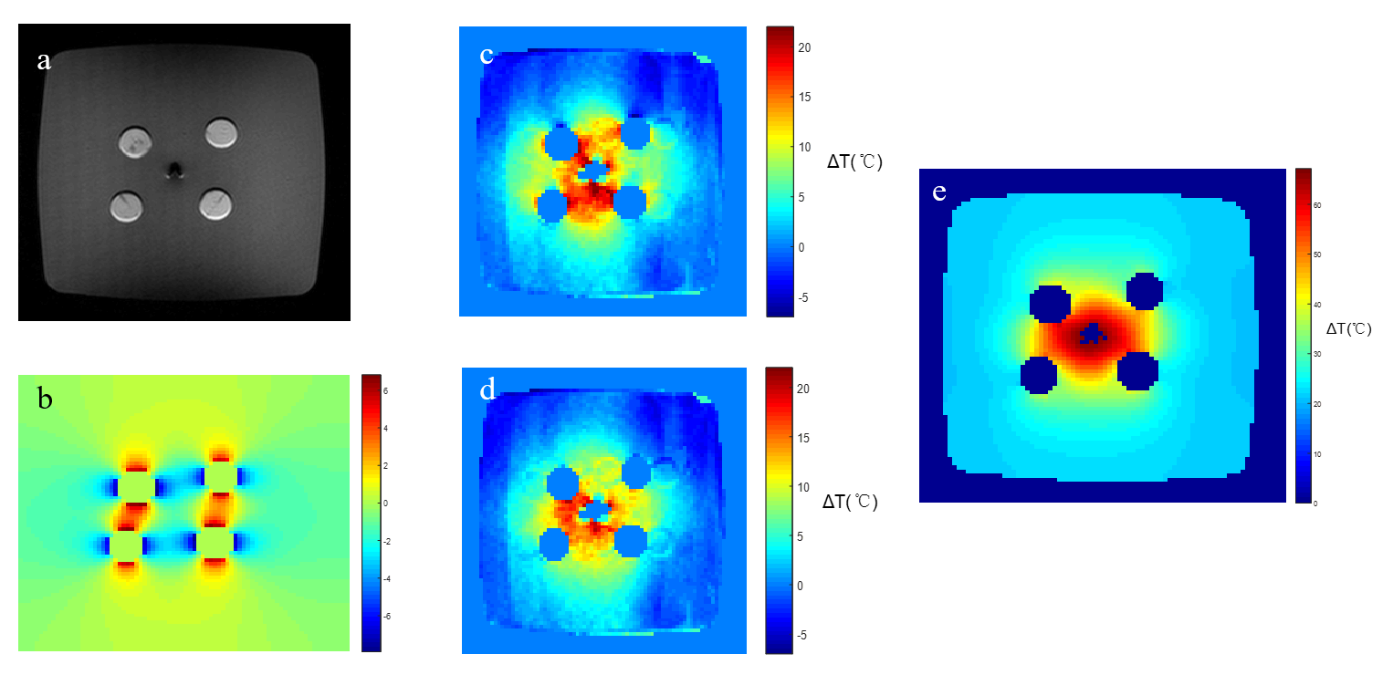
A phantom experiment was also conducted to validate the accuracy of fat temperature monitoring by VFA method. The phantom consisted of a rectangular water gel (150×150×60mm3, 1% agar) with four lard oil cylinder (radius = 8.5mm, length = 60mm) placed inside. The scan parameters were the same as the third experiment , except only two different flip angles 4°/20° were used.
Results
The results of the first two phantom experiment are shown in Fig.2 and Fig.3. Large temperature errors up to 1.2$$$^\circ C$$$ and 3.8$$$^\circ C$$$ can be observed in the location of the optical fiber respectively in two experiments and the corrected temperature achieved better matching to the real temperature measured by optical fibers.
The results of the calibration experiment are shown in Fig.4. that although noisy, the T1 measurements displayed a linear temperature dependence in lard oil. The slope was found to be 1.982 $$$ms$$$/$$$^\circ C$$$.
The results of the phantom heating experiment are shown in Fig.5. After correction, the temperature changes in the areas near fat cylinder were much close to the simulated real temperature changes map.
Discussion and Conclusion
According to the result, both phantom experiments validated the estimation of the proposed algorithm based on Maxwell’ s Equation for the corrected temperature was much more close to the real temperature especially near the fat tissues. In addition, the method which can monitor water and fat tissues simultaneously has been proved to be accurate enough to be utilized in the temperature-induced susceptibility correction method.Acknowledgements
This work is supported by National Natural Science Foundation of China: NSFC 6177010624.References
[1]Sprinkhuizen SM, Konings MK, van der Bom MJ et al.Temperature-Induced Tissue Susceptibility Changes Lead to Significant Temperature Errors in PRFS-Based MR Thermometry During Thermal Interventions[J]. Magnetic Resonance in Medicine , 2010, 64: 1360-1372.
[2] Kressler B, Rochefort L, Liu T, et al.Nonlinear Regularization for Per Voxel Estimation of Magnetic Susceptibility Distributions from MRI Field Maps[J]. IEEE Trans Med Imaging, 2010, 29(2): 273-281.
[3] Rochefort L, Liu T, Kressler B et al. Quantitative Susceptibility Map Reconstruction from MR Phase Data Using Bayesian Regularization: Validation and Application to Brain Imaging[J]. Magnetic Resonance in Medicine , 2010, 63(1): 194-206.
[4] Todd N, Diakite M, Payne A et al. Hybrid proton resonance frequency/T1 technique for simultaneous temperature monitoring in adipose and aqueous tissues. Magn Reson Med 2013;69:62–70.
Figures