1453

The transfer function for implanted wires when a second wire is near.

Peter R.S. Stijnman¹, Janot P. Tokaya¹, Cornelis A.T. van den Berg¹, and Alexander J.E. Raaijmakers¹

¹Center for Image Sciences, UMC Utrecht, Utrecht, Netherlands

Synopsis

Lead wires of medical implants can pose a severe safety risk due to RF-induced heating. Risk assessment typically involves determination of the transfer function. This study shows that the transfer function may drastically change if a second wire is located close to the lead wire. An explorative simulation study has been performed investigating the impact of inter-wire spacing and wire length on the alteration of the transfer function by the second wire. Results reveal that in particular insulated wires may show very strong enhancements (>100%) in induced currents if a second wire is present.

Introduction

For active implantable medical devices, the lead wires pose the biggest safety risk in terms of RF induced heat generation. Typically, the risk for heating is evaluated by use of the transfer function (TF)¹. Transfer functions describe the electric field enhancement at the tip of an implant due to excitation by a tangential electric field distribution along the implant. However, the presence of other conductive structures surrounding the implant lead (e.g. a second wire) may drastically alter the TF and, thereby, the expected heating level. In this work the effects of a second wire on the TFs of a single lead wire are investigated with electromagnetic simulations at 1.5T and 3T.

Methods

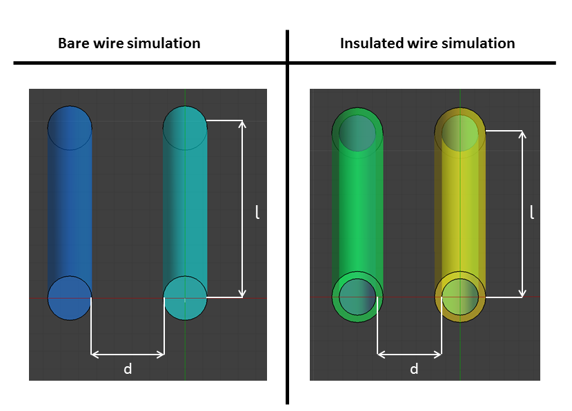
Figure 1 depicts the setup for the electromagnetic simulations (Sim4Life,ZMT,Zurich). To investigate the impact of inter-wire spacing ($$$d$$$) on the TF, determined with an excitation at its tip exploiting the principle of reciprocity², for different $$$d$$$ (ranging from 1mm to 12mm) and a constant wire length ($$$l$$$) of 20cm. This data was acquired for bare and isolated wires at 1.5T and 3T. A second simulation series was performed to determine the TF for a double wire setup as a function of the $$$l$$$, ranging from 10 till 40cm, with $$$d$$$ kept constant at 5mm. Again, the TFs were determined for bare and isolated wires at 1.5T and 3T. A hard source (1V/m amplitude) was used to excite the first lead wire, the second wire was not excited.

Results & Discussion

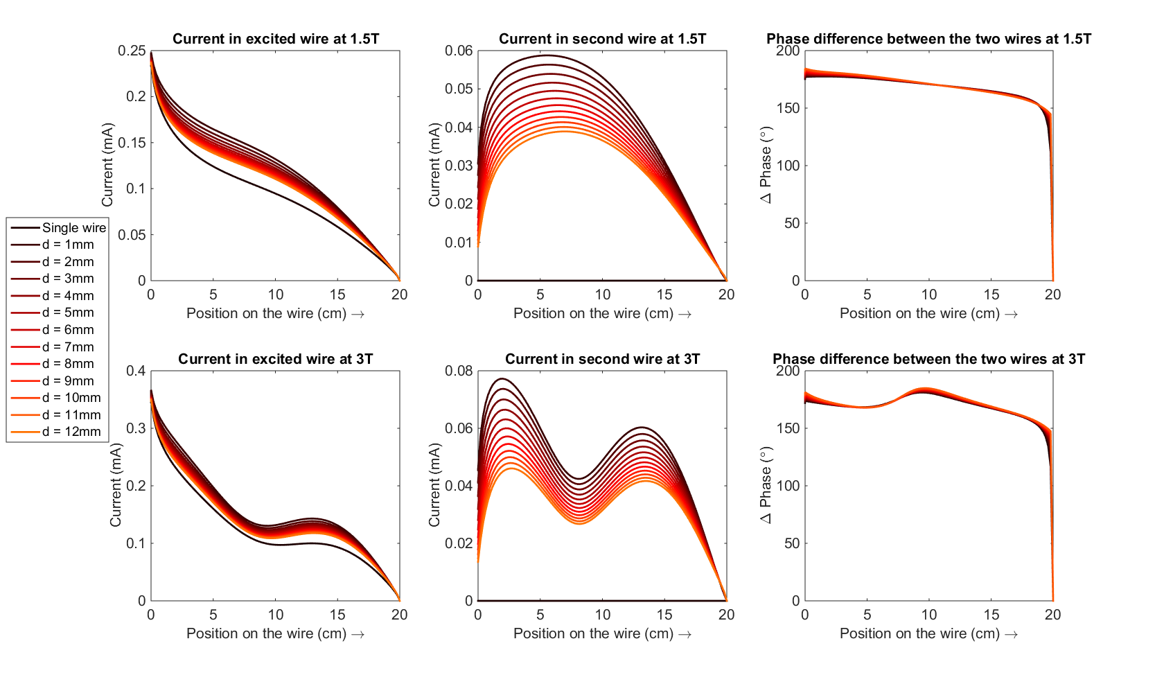
Figures 2a and d show the current distributions in the first wire which are effectively the TFs for those setups. Strikingly, the current distribution along the wire increases when the second wire is present. When $$$d$$$ increases the current distribution along the wire decreases and tends towards the current distribution when the second wire is not present. Figures 2b and e show the current induced in the second wire, when $$$d$$$ increases the induced current decreases as expected. Figures 2c and f show the phase difference between the wires, which is close to $$$180^\circ$$$, meaning the currents are running in opposite directions.

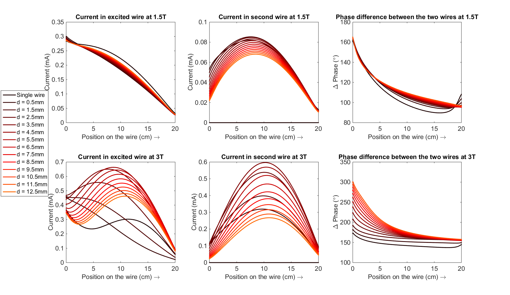
Figure 3 shows equivalent plots for the insulated wires. Figure 3a shows that the presence of the second wire at 1.5T reduces the overall current distribution of the excited wire. Figure 3b shows that the current distribution induced in the second wire decreases with $$$d$$$, although the amplitude for the smallest value for $$$d$$$ (0.5mm) actually shows a slightly lower value than at 1.5mm. The maximum induced current amplitude is 27% of the current amplitude in the first wire. However, at 3T the pattern is essentially different. Figure 3d shows that the presence of the second wire drastically increases the current in the first wire, by 109%. Figure 3e shows that the maximum current amplitude in the second wire is 90% of the maximum current amplitude in the excited wire. This increase in current does not occur in the bare wire simulations because the currents are strongly attenuated due to current leakage to the conductive surrounding. Figures 3c and f show that the phase difference between the two wires varies along $$$l$$$.

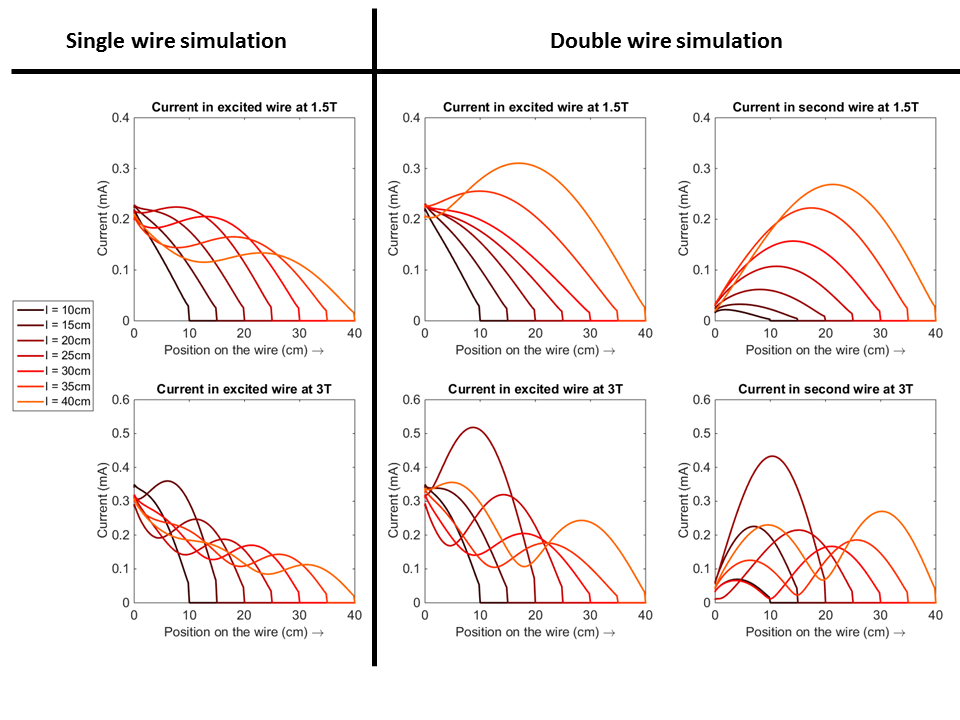
Figure 4 shows the simulations when $$$l$$$ is varied and $$$d$$$ is kept constant. In Figure 4a and d the current distributions for the single wire simulations are shown. From figures 4b,c,e and f resonance lengths are visible as highly increased currents that occur at specific wire lengths, which are 40cm for 1.5T (132% increase in maximum current) and 20cm for 3T (109% increase in maximum current).

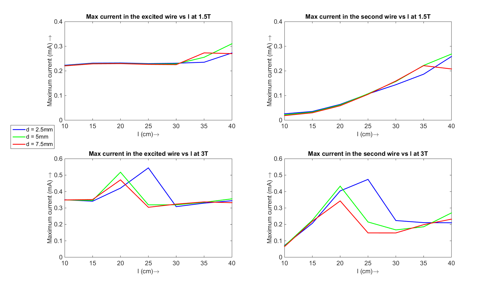
After both varying $$$l$$$ and $$$d$$$ separately Figure 5 shows the maximum current for different $$$d$$$ plotted against $$$l$$$, for 1.5T and 3T and for the excited and second wire (only for insulated wires). In the 1.5T simulations the maximum current for $$$d = 7.5mm$$$ occurs at a wire length of 35cm, whereas for smaller inter-wire spacing the resonance length increases. From the simulations at 3T a similar dependence is observed. From the 3T simulations it is observed that the maximum current at the resonance length increase for the smaller inter-wire spacing, which was also observed in Figures 2 and 3.

Conclusion

From the results that are shown in Figures 2 through 5 it is evident that the presence of a second wire changes the TFs of the single lead wire. This may increase or decrease the current along the wire. For insulated wires more than doubling of the maximum current is shown, which poses a severe safety risk if wires are routed in such fashions through the patient without precaution.

Acknowledgements

This research is supported by NWO, Medtronic and Philips. Further the authors would like to thank Arcan Ertürk for interesting discussions.

References

[1] S.M. Park, R. Kamondetdacha, J.A. Nyenhuis, Calculation of MRI-inducedheating of an implanted medical lead wire with an electric field transfer function. JMRI, 2007. DOI: 10.1002/jmri.21159

[2] S. Feng, R. Quing, W. Kainz, J. Chen, A technique to evaluate MRI-Induced Electric Fields at the Ends of Practical Implanted Lead, IEEE, 2015. DOI: 10.1109/TMTT.2014.2376523

Figures

Figure 1: The left figure shows the 3D-FDTD simulation setup for bare copper wires. The inter-wire distance is indicated by $$$d$$$ and the length of the wire with $$$l$$$. The right wire is excited using a hard source at the tip of the wire while the left wire has no source attached to it. The right figure show the simulation setup for the insulated copper wires. The radius of the wires is 1.25mm, the insulation thickness is 0.5mm and its relative permittivity 5. The background used for the simulations was a dielectric of conductivity 0.35S/m and relative permittivity of 78.

Figure 2: The top row shows the simulations at 1.5T, where the figure shows the current distribution for the excited wire for different $$$d$$$. The middle figure shows the current distribution for the second wire and the right figure depicts the phase difference between the two wires. The bottom row is analogous to the top row accept for the field strength of 3T.

Figure 3: The top row show the currents in the wires from simulation at 1.5T, where the left figure shows the current distribution along the excited insulated wire for different $$$d$$$. The middle figure shows the current distribution along the second insulated wire and the right figure depicts the phase difference between the two wires. The bottom row is analogous to the top row accept for the field strength of 3T.

Figure 4: The top row shows the simulations at 1.5T, where the left figure depicts the current distribution in the excited insulated wire for different lengths in a single wire simulation. The middle figure shows the current distribution in the excited insulated wire for different lengths when a second wire is present at $$$d = 5mm$$$. The figure on the right shows the current distribution in the second wire. The bottom row is analogous to the top row accept for the field strength of 3T.

Figure 5: The top row shows the maximum current in the excited insulated wire (left figure) and the second insulated wire (right figure) at 1.5T for different wire lengths. The inter-wire distance was varied from 2.5mm to 5mm to 7.5mm. The bottom row is analogous to the top row accept for the field strength of 3T.

Proc. Intl. Soc. Mag. Reson. Med. 26 (2018)

1453