Synopsis

We examine how Machine Learning can be used to identify novel risk factors of osteoporotic bone fracture. Using measurements from patient MRI scans at five anatomical sites, we sought to find which specific regions are best for stratifying the risk of osteoporotic fracture. Further studies on these models and other data will help improve clinicians’ ability to accurately diagnose Osteoporosis, so that patients at risk for bone fracture may be caught and treated earlier.

Introduction

Osteoporosis is a debilitating disease which can lead to a higher incidence of bone fracture. However, treatments are prescribed to patients that meet osteoporotic diagnostic criteria irrespective of fracture status. As a result, some patients with fractures may go untreated while others that may never have a fracture will go over-treated. MRI technological advances have brought added diagnostic power to many diseases, including musculoskeletal ones. The parameters it provides can be sensitive to microstructural changes in the bone, which in turn may be useful for predicting fracture risk. As is apparent from previous musculoskeletal [2, 3] and neuroimaging studies [4], one popular application of Machine Learning is in classification.

In this study we:

• compare different Machine Learning techniques for prediction of osteoporotic bone fractures based on data that include MRI parameters;
• apply Neighborhood Component Analysis (NCA) and univariate analysis for feature selection; and
• offer a comparison of the two above techniques across various anatomical bone regions.

Methods

The dataset includes 92 subjects who presented for high-resolution 3T MRI examination of the proximal femur ( D-FLASH, TR/TE=37ms/4.92ms, flip angle=25􏰔 , bandwidth = 130Hz/pixel, FOV=100mm, matrix=512x3x512, voxel=0.234x0.234x1.5 mm, parallel imaging (GRAPPA) factor = 2, scan-time=15min) of whom 32 had prior fragility fractures and 60 did not. Microstructural MRI measures of bone quality were obtained via topological analysis, as described in the original paper by Saha et al. [8], in five 10x10x10mm^3 volumes of interest within the femoral head, neck, Ward’s triangle, greater trochanter, and intertrochanteric region.
We construct multiple datasets via bootstrapping, to simulate real-world noise, and investigate the stability of predictions. These datasets are created by randomly sampling data points from the original dataset; the points left out are used for testing the model fitting [7].

Because some pairs/groups of features within the complete set of parameters may provide similar information, we use two techniques to select subsets that are least redundant/most informative. This gives three sets:

• All features: The first dataset includes all the predictors associated with this dataset: age, weight, height, and MRI parameters.
• NCA: a non-parametric dimensionality reduction method used on K-nearest neighbors (KNN) classification algorithms [5]. We use it on the MRI-derived features only.
• univariate: in this standard and established method, for each feature/covariate, we fit a univariate logistic regression model [6].

To these datasets we fit three models: Logistic Regression (LG, a binomial logistic regression model), Naive Bayes (NB, where the prior and likelihood are found on the training data, while the posterior distribution is calculated on the unseen testing data), and Support Vector Machine (SVM, which aims to classify data by finding the hyperplane that separates the responses with the highest possible margin).

The performance of the models is evaluated using:

• accuracy=((TN+FP)/(TN+FP+FN+TN))
• sensitivity=(TPR=TP/(TP+FN))
• specificity (TNR=TN/(TN+FP))
• adjusted accuracy=accuracy+sensitivity+specificity-|sensitivity-specificity|

which are defined via fractions of real (true positives, TP) or misidentified (false positives, FP) fracture cases; and non-fracture cases, whether real (true negative, TN) or not (false negative, FN).

Results

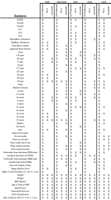
Fig.1 shows the features selected across the datasets of different anatomical regions. There is wide variability across the sets and the NCA and univariate techniques.

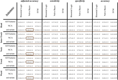
Fig.2 shows that the Naïve Bayes model gives better adjusted accuracy (via both reduced feature sets), as encircled in the first column of the figure. The Support Vector Machine, while being the best in specificity, is also the worst in sensitivity. Across the five anatomical regions, the inter-trochlear region provides the highest adjusted accuracy on the NCA selected features.

Discussion:

The dataset is not a random sampling of a normal population, and the small sample size may bias the estimation of the specificity and the sensitivity indices. It is for this reason that this work uses bootstrapping/CV to alleviate the inherent bias in estimating the model parameters and making predictions [9]. Future work will examine this further.

Conclusion

Acknowledgements

References

1. Frederick H Hooven, Jonathan D Adachi, Silvano Adami, Steven Boonen, J Compston, Cyrus Cooper, Pierre Delmas, Adolfo Diez-Perez, S Gehlbach, Susan L Greenspan, et al., “The global longitudinal study of osteoporosis in women (glow): rationale and study design,” Osteoporosis international, vol. 20, no. 7, pp. 1107–1116, 2009.
2. Christian Kruse, Pia Eiken, and Peter Vestergaard, “Machine learning principles can improve hip fracture prediction,” Calcified tissue international, vol. 100, no. 4, pp. 348–360, 2017.
3. Guillaume Madelin, Frederick Poidevin, Antonios Makrymallis, and Ravinder R Regatte, “Classification of sodium MRI data of cartilage using machine learning,” Magnetic Resonance in Medicine, vol. 74, no. 5, pp. 1435– 1448, 2015.
4. V Wottschel, DC Alexander, PP Kwok, DT Chard, ML Stromillo, N De Stefano, AJ Thompson, DH Miller, and O Ciccarelli, “Predicting outcome in clinically iso- lated syndrome using machine learning,” NeuroImage: Clinical, vol. 7, pp. 281–287, 2015.
5. Jacob Goldberger, Geoffrey E Hinton, Sam T Roweis, and Ruslan R Salakhutdinov, “Neighbourhood components analysis,” in Advances in neural information processing systems, 2005, pp. 513–520.
6. David W Hosmer Jr, Stanley Lemeshow, and Rodney X Sturdivant, Applied logistic regression, vol. 398, John Wiley & Sons, 2013.
7. Bradley Efron and Robert Tibshirani, “Improvements on cross-validation: the 632+ bootstrap method,” Journal of the American Statistical Association, vol. 92, no. 438, pp. 548–560, 1997.
8. Punam K Saha, Bryon R Gomberg, and Felix W Wehrli, “Three-dimensional digital topological characterization of cancellous bone architecture,” International Journal of Imaging Systems and Technology, vol. 11, no. 1, pp. 81–90, 2000.
9. David Colquhoun, “An investigation of the false discovery rate and the misinterpretation of p-values,” Royal Society open science, vol. 1, no. 3, pp. 140216, 2014.