1324
Spectral Quantification for Multiple-TE Spectroscopy Using Spectral Priors and Measured Lineshape Distortion Function1Beckman Institute for Advanced Science and Technology, University of Illinois at Urbana-Champaign, Urbana, IL, United States, 2Department of Electrical and Computer Engineering, University of Illinois at Urbana-Champaign, Urbana, IL, United States
Synopsis
This work presents a new method for quantifying multiple-TE/two-dimensional spectroscopy data, characterized by the use of spectral priors obtained by quantum mechanical simulations and an experimentally measured lineshape distortion function derived from a set of multi-TE water spectroscopic data. Results from in vivo J-resolved spectroscopy data demonstrated the excellent fitting produced by the proposed method, and improved robustness over a standard parametric-model-based method. With further developments, such as extensions to different sequences and Cramer-Rao bound analysis, the proposed method should prove useful for a range of 2D spectroscopy experiments.
INTRODUCTION
Multiple-TE or J-resolved spectroscopy offers improved detection and quantification of various molecules, especially for J-coupled molecules with strong spectral overlap in a single spectral dimension1-4. However, the quantification of multi-TE spectroscopy data remains challenging, due to the increased modeling complexity needed to capture the spectral variations along both the chemical-shift and TE dimensions as well as the presence of experiment-dependent signal distortion5,6. Thus, most studies nowadays are limited to a TE-by-TE one-dimensional quantification followed by subsequent corrections and analysis7. We present here a new method for quantifying multi-TE spectroscopy data, characterized by the use of spectral priors to reduce the degrees-of-freedom and the incorporation of an experimentally measured lineshape distortion function. The proposed method has been evaluated using in vivo single-voxel J-resolved spectroscopy data, which demonstrated excellent fitting with improved robustness over a conventional parametric-model-based method.THEORY&METHODS
Signal Model
To address the key issues of modeling the spectral variations of individual molecules at different TEs and accounting for signal distortion for multi-TE quantification, we propose to use the following model (also considering sampling before echoes)
$$s(t,TE_i) = \sum_{m=1}^{M}a_m\phi_{m,i}(t,\tau_i)e^{-(TE_i-TE_1)/T_{2,m}}e^{-(t-\tau_i)/T_{2,m}}e^{i2\pi\delta f_m(t-\tau_i)}e^{-i\theta_{m,i}+i2\pi\Delta f_{i}t}h_i(t) + \sum_{b=1}^{B}c_b\phi_b(t,TE_i)e^{-\beta_bt}, \quad [1]$$
where $$$TE_i$$$ denotes the $$$i$$$th echo time, $$$t$$$ the free-precession time, $$$a_m$$$ the molecular concentration, and $$$\{\tau_i\}$$$ the sampling periods before echoes. Spectral priors are incorporated through the resonance structures $$$\{\phi_{m,i}(t)\}$$$ (from quantum mechanical simulations) and exponential lineshapes only dependent on molecular-specific parameters, i.e., relaxation parameters $$$T_{2,m}$$$ and frequency shifts $$$\delta f_m$$$. The additional terms $$$\theta_{m,i}$$$ and $$$\Delta f_{i}$$$ account for phase discrepancy and field shifts across TE. Finally, the time-domain envelope function $$$h(t)$$$ is used to model the experiment-dependent lineshape distortions (e.g., due to intra-voxel B0 inhomogeneity and/or eddy currents). The last summation captures the baseline with basis $$$\{\phi_b(t)\}$$$ and damping factors $$$\{\beta_b\}$$$.
Distortion Estimation
A key component in the proposed method is the determination of $$$h(t)$$$. Existing methods typically model $$$h(t)$$$ by Gaussian functions with additional phase terms, and try to jointly determine the associated nonlinear parameters from the data, increasing the number of unknowns for fitting. We propose here a different approach to address this, by acquiring a set of water spectroscopic signals with selected TEs from the same voxel (this can be done quickly since only one average per TE is needed). Specifically, we model the water data as
$$s_w(t,TE_i) = e(TE_i; T_{2,w})e^{-t/T_{2}'+i2\pi f_0t}\sum_{l=-L/2+1}^{L/2}\alpha_le^{i2\pi l\Delta ft}, \qquad\qquad\qquad\qquad\qquad\qquad [2]$$
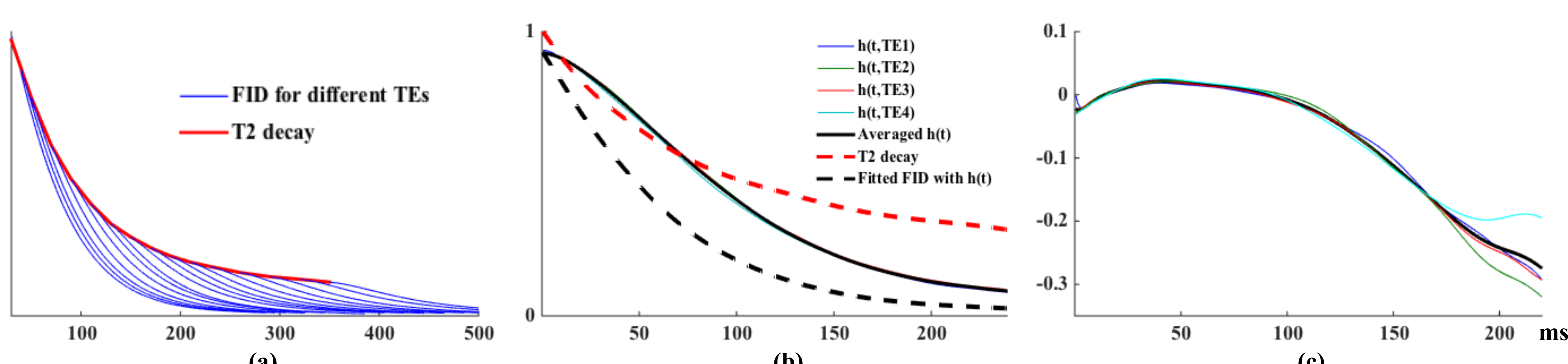
where $$$e(TE_i; T_{2,w})$$$ captures pure $$$T_2$$$-dependent signal decay, $$$e^{-t/T_2'}$$$ and $$$f_0$$$ the exponential decay and frequency shift caused by intra-voxel B0 inhomogeneity, respectively, and the last term models the non-exponential distortion. While separating $$$e(TE_i; T_{2,w})$$$ from $$$e^{-t/T_2'}$$$ from a single FID is highly ill-posed, the problem becomes simpler with the multi-TE water data available. More specifically, the samples at echo times from the water FIDs (denoted as $$$\{s_w(t=0,TE_i)\}$$$) can be used to extract the $$$T_2$$$-decay, by interpolating $$$\{s_w(0,TE_i)\}$$$ to the FID sampling grids (e.g., using a spline kernel). This interpolation is accurate given a sufficient number of TEs and more robust than a multi-$$$T_2$$$ parametric fitting which suffers from poor-conditioning.
With $$$e(.)$$$ determined, it is incorporated into Eq. [2] for the fitting of $$$s_w(t,TE_i)$$$ to determine $$$T_2'$$$, $$$f_0$$$ and $$$\{\alpha_l\}$$$. TE-dependent $$$h(t)$$$'s were synthesized in the form of $$$e^{-t/T_{2}'}\sum\alpha_le^{i2\pi l\Delta ft}$$$ and averaged to generate the final estimate, which was then incorporated into Eq. [1] for the proposed multi-TE quantification. The fitting was done by solving a least-squares problem using a variable-projection-based algorithm.
RESULTS AND DISCUSSION
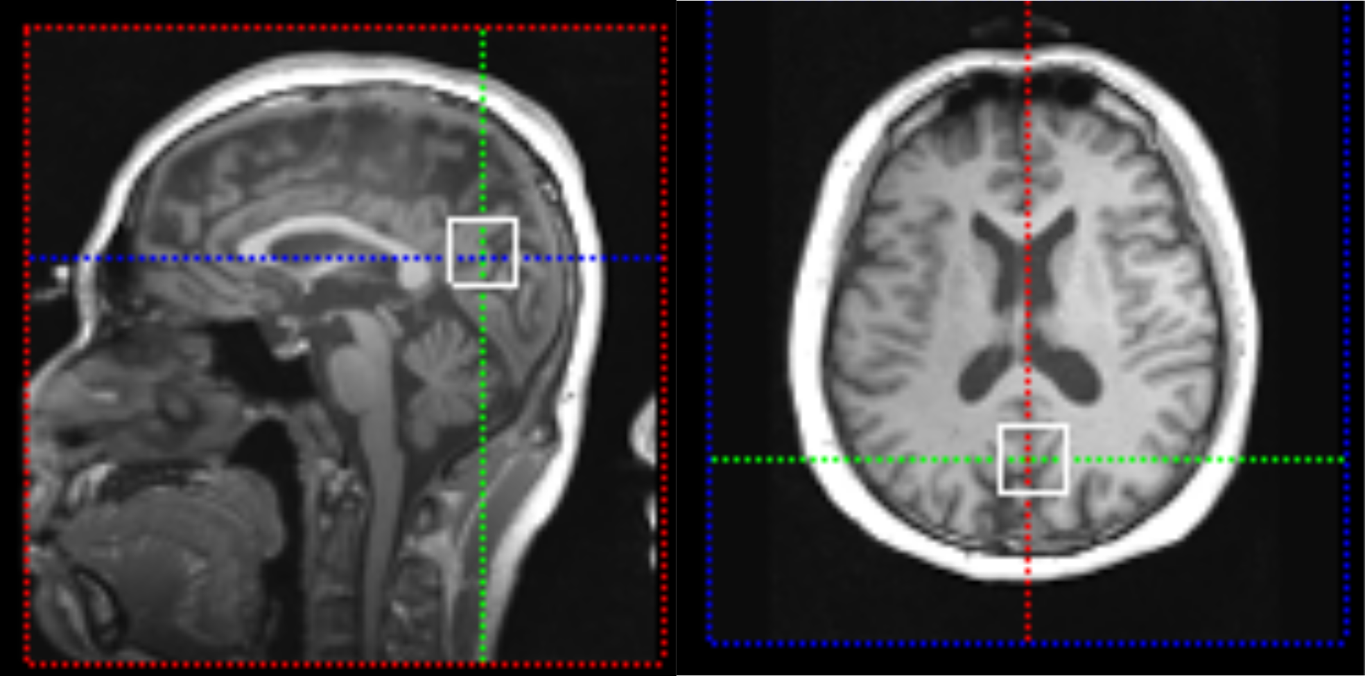
In vivo localized J-resolved data were acquired to evaluate the proposed method. Data were acquired on a 3T scanner (Siemens Prisma) using a PRESS sequence. Water-suppressed data were acquired from 20x20x20mm3 voxels with TE=30,80,160ms1, TR=2500ms, 100 averages, 2kHz bandwidth, and 512 FID samples. The voxel location is illustrated in Fig. 1. Water data were acquired at 16 TEs ranging from 30 to 350ms (optimized by simulations of sampling a signal with 3 TE components) and TR=4s.
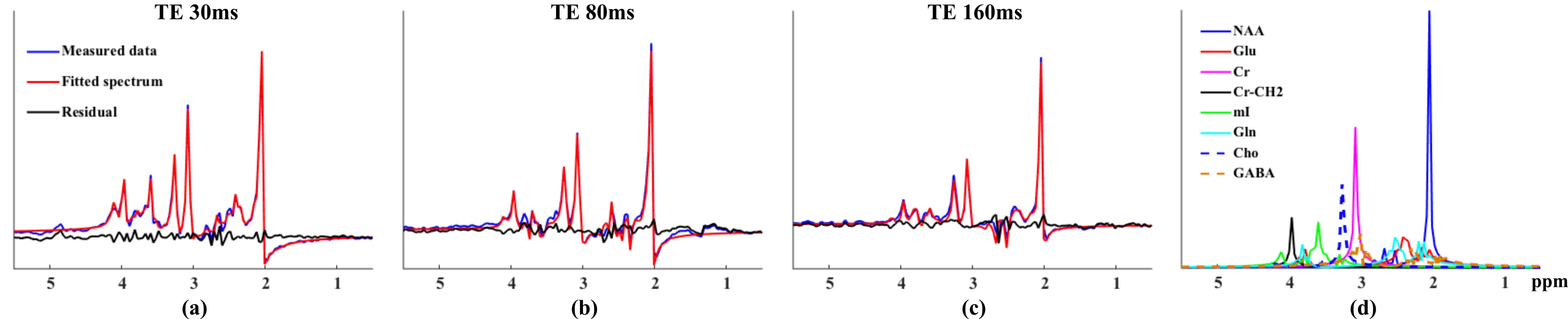
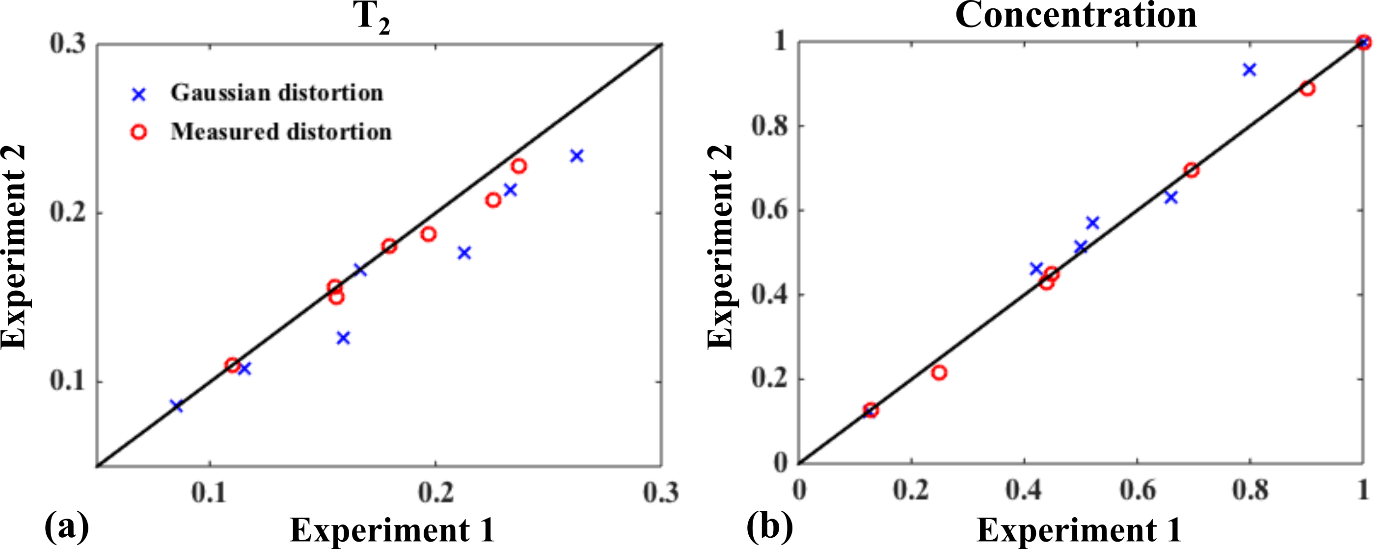
Figure 2 shows the processing results for the water data, particularly the successful estimation of $$$e(TE_i;T_{2,w})$$$ and $$$h(t)$$$. Figure 3(a)-(b) show the fitting results for different TEs from a representative dataset. Small residuals are observed. Separated individual metabolite components are shown in Fig. 3(d). Figure 4 compares the estimated parameters from two repeated experiments on the same subject. As can be seen, the parameters produced by the proposed method are clearly more reproducible than a standard parametric model which uses the Voigt lineshapes1.
CONCLUSION
We presented a new method for quantifying multi-TE spectroscopy data, characterized by the use of molecular-specific spectral priors and an experimentally measured lineshape distortion function. Experimental results demonstrated the effectiveness of the proposed method. With further developments, the proposed method should prove useful for a range of 2D spectroscopy experiments.Acknowledgements
This work is supported in parts by NIH-R21-EB021013-01 and NIH-P41-EB002034.References
1. Bolliger CS, Boesch C, and Kreis R, On the use of Cramer–Rao minimum variance bounds for the design of magnetic resonance spectroscopy experiments. NeuroImage, 2013;83:1031-1040.
2. de Graaf RA, In vivo NMR spectroscopy: Principles and techniques. Hoboken, NJ: John Wiley and Sons, 2007.
3. Ryner LN, Sorenson JA, and Thomas MA, 3D localized 2D NMR spectroscopy on an MRI scanner. J. Magn. Reson., 1995;107:126-137.
4. Li Y, Chen AP, Crane JC, Chang SM, Vigneron DB, and Nelson SJ, Three-dimensional J-resolved H-1 magnetic resonance spectroscopic imaging of volunteers and patients with brain tumors at 3T. Magn. Reson. Med., 2007;58:886-892.
5. Schulte RF and Boesiger P, ProFit: two-dimensional prior-knowledge fitting of J-resolved spectra. NMR Biomed., 2006;19:255-263.
6. Fuchs A, Boesiger P, Schulte RF and Henning A, ProFit revisited. Magn. Reson. Med., 2014;71:458-468.
7. Provencher SW, Automatic quantitation of localized in vivo 1H spectra with LCModel. NMR Biomed., 2001;14:260-264.
Figures