1323

Metabolite quantitation using water-scaling corrected with Magnetic resonance fingerprinting

Ryan J Larsen¹, Joseph L. Holtrop^1,2, and Brad P. Sutton^1,2

¹Beckman Institute, University of Illinois at Urbana-Champaign, Urbana, IL, United States, ²Department of Bioengineering, University of Illinois at Urbana-Champaign, Urbana, IL, United States

Synopsis

Quantitation of MRSI data using water-scaling requires correction of the water signal for relaxation and CSF partial volume effects. We demonstrate the use of a rapid MRF sequence to characterize the water signal used to quantify MRS data, which we call WAter-scaling Quantification using MRF (WAQ-MRF) scan. WAQ-MRF provides subject-specific corrections of partial volume and relaxation effects for water-scaled data. By adding a one minute scan to a standard MRSI acquisition it is possible to eliminate the need for assuming literature values of relaxation and proton density to correct the water signal.

Introduction

Quantitation of MRSI data using water-scaling requires correction of the water signal for relaxation and CSF partial volume effects. Here we demonstrate the use of a rapid MRF [1] sequence to characterize the water signal used to quantify MRS data, which we call WAter-scaling Quantification using MRF (WAQ-MRF) scan. The technique consists of rapid acquisitions of multiple MRSI scans using a series of random values of TE and TR.

Methods

Our implementation of WAQ-MRF consists of a single-slice PRESS excitation (90° flip angle, 100 x 100 mm, thickness 20 mm), followed by a single-shot spiral readout (FOV: 200 x 200 ms, 16 x 16 matrix size). The sequence consists of 20 acquisitions; the first of which is played with TE = 30 ms and TR = 20 s to ensure full relaxation. Values of TE for the remaining acquisitions are chosen from a random permutation of 19 logarithmically spaced values from TE = 30 ms to 1000 ms. Values of TR are selected randomly on a logarithmical scale from the minimum TR allowed, to 4000 ms. The seven WAQ-MRF sequences used for this study ranged from 52 to 56 seconds.

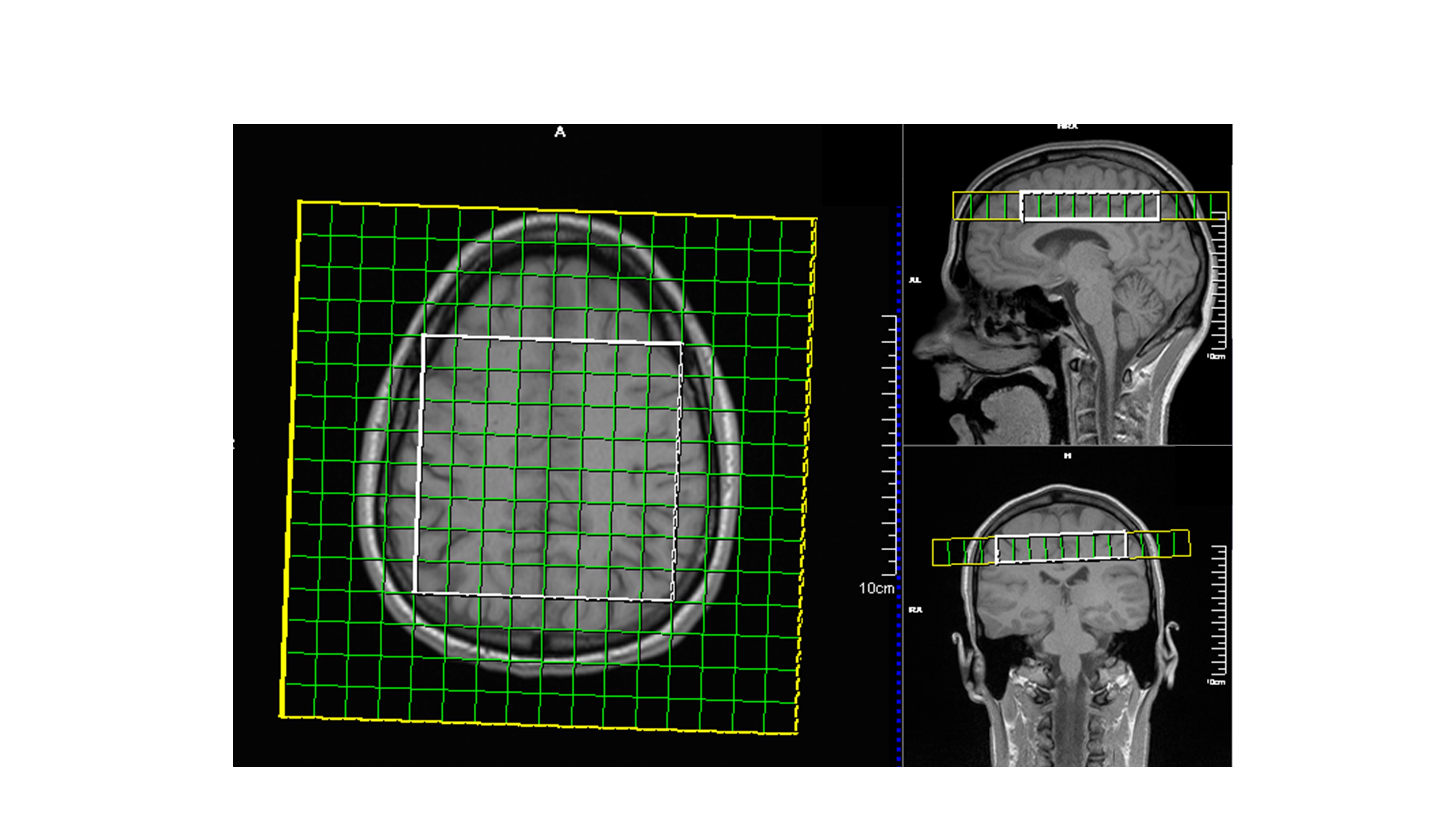
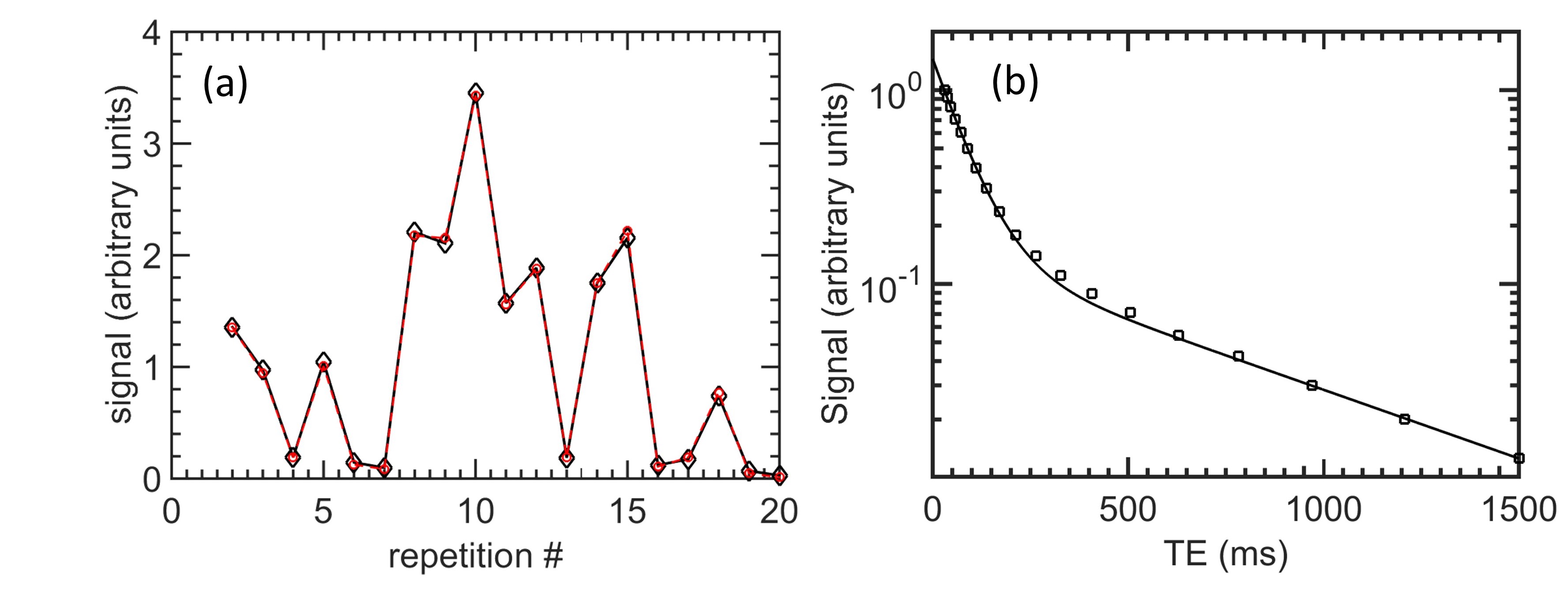
Data were acquired on four human volunteers, with IRB approval, using a Siemens TIM Trio 3 T system with a 12-channel or 32-channel head coil. The imaging slice was oriented axially, superior to the lateral ventricles (Fig. 1). Images were reconstructed using gridding. The magnitude of the signal at the echo time of each repetition was fit in the least squares sense as a linear combination of the results of Bloch simulations of CSF and brain tissue relaxation, stored in look-up tables (Fig. 2(a)). MRS spectra were measured using a double phase-encoded PRESS sequence over the same volume as the WAQ-MRF sequence (Region of Excitation: 100 x 100 mm, FOV: 200 x 200, TR/TE = 2000/30 ms, 16 x 16 matrix size, elliptical sampling, spectral bandwidth 2000 Hz, 90° flip angle, saturation bands along all six edges of the excitation region, one average with water suppression, followed by a second scan without water suppression). A structural scan was also obtained, (MPRAGE, FOV: 230 x 230 mm, TR/TE = 1900/2.32 ms, Inversion time 900 ms, 0.9 mm isotropic resolution, GRAPPA factor of 2). We estimated the molar concentration of metabolite, $$$M$$$, using the ratio of metabolite signal to water signal $$$S_M/S_W$$$ according to

$$[M] = \frac{2}{H_M} \frac{R_W}{R_M(1-f_{CSF})}\frac{S_M}{S_W}[W]$$

where is the number where $$$H_M$$$ is the number of protons in the metabolite, $$$[W]$$$ is the neat water concentration, $$$f_{CSF}$$$ is the mole fraction of CSF, and the $$$R$$$ factors account for relaxation of the metabolite and water signal.[2] Water relaxation, $$$R_w$$$, is given by $$R_W = \sum_{i} f_i \exp{(-TE/T_{2i})}(1-\exp{[-TR/T_{1i}]})$$ where $$$f$$$ is the mole fraction of water, and the subscript $$$i$$$ refers to compartment $$$i$$$.

For comparison to a different method [2], we also computed metabolite concentration maps, $$$[M]_{SEG}$$$, using tissue segmentation into three compartments (white matter –WM, grey matter –GM, and CSF) together with literature values of $$$T_1$$$ and $$$T_2$$$,[3-5] and proton density [6] in each of the three compartments. For two of the subjects, we also performed an additional acquisition in which the WAQ-MRF sequence was performed under fully relaxed conditions (Fig. 2(b)).[7]

Results

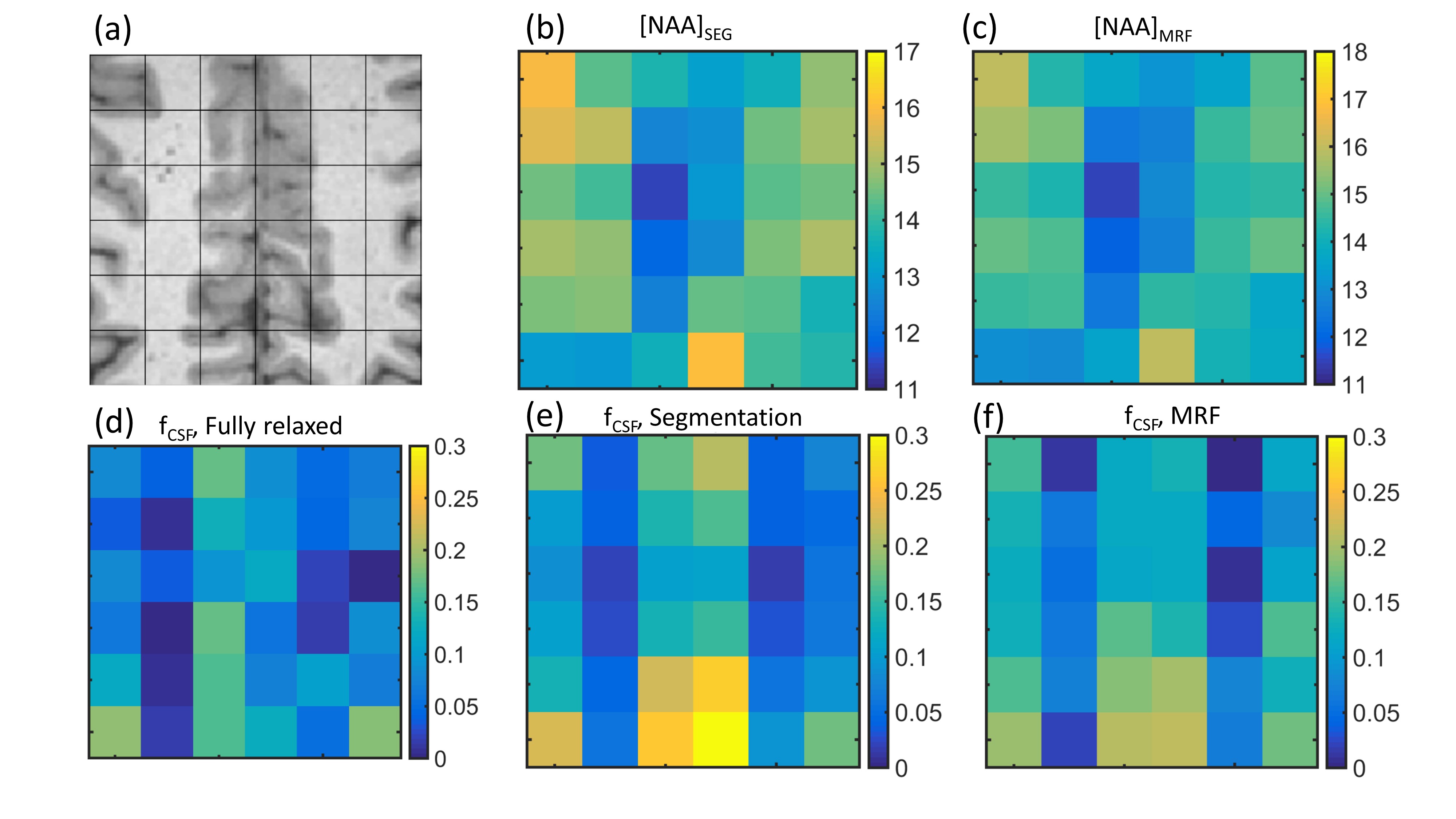
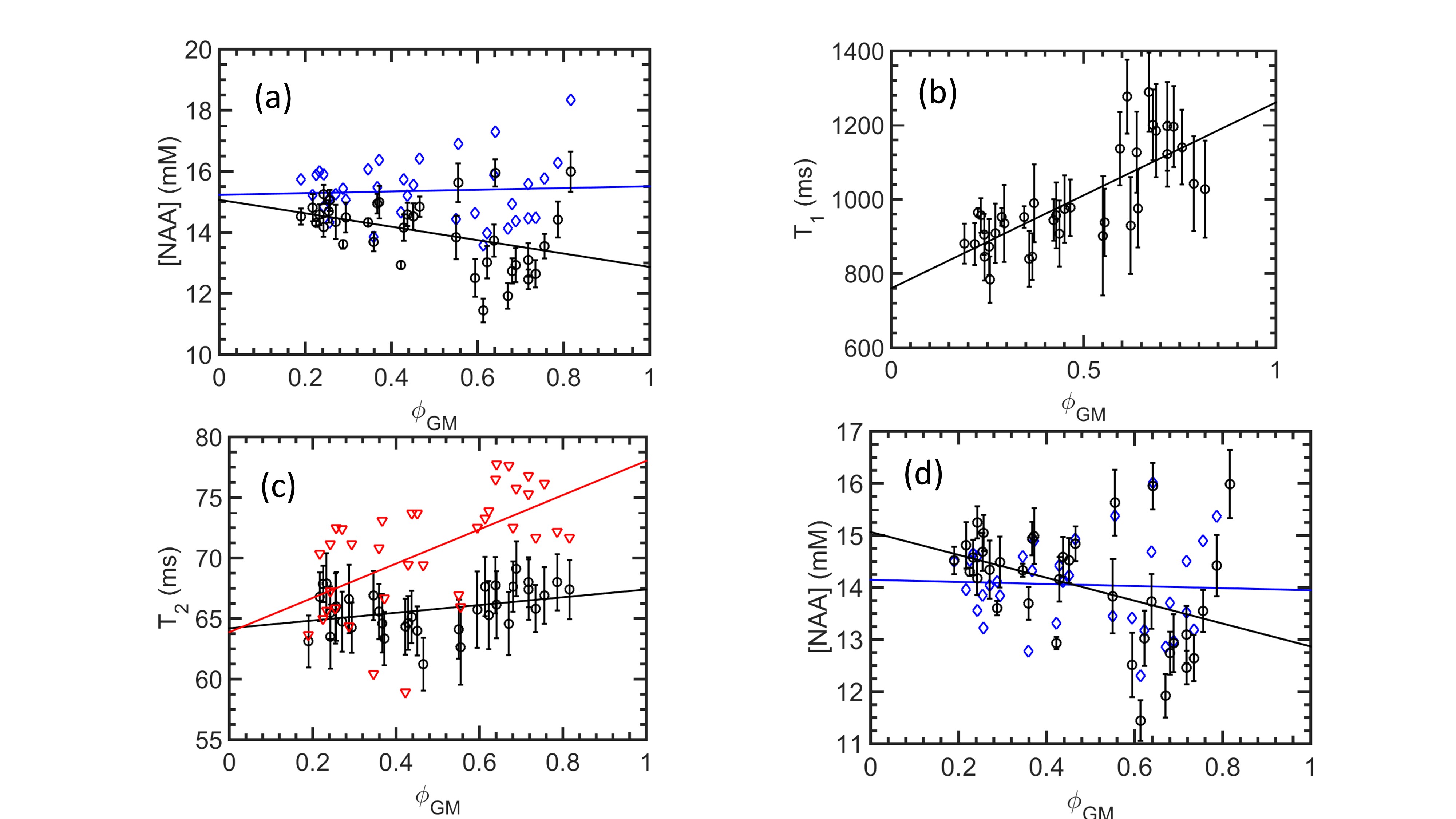
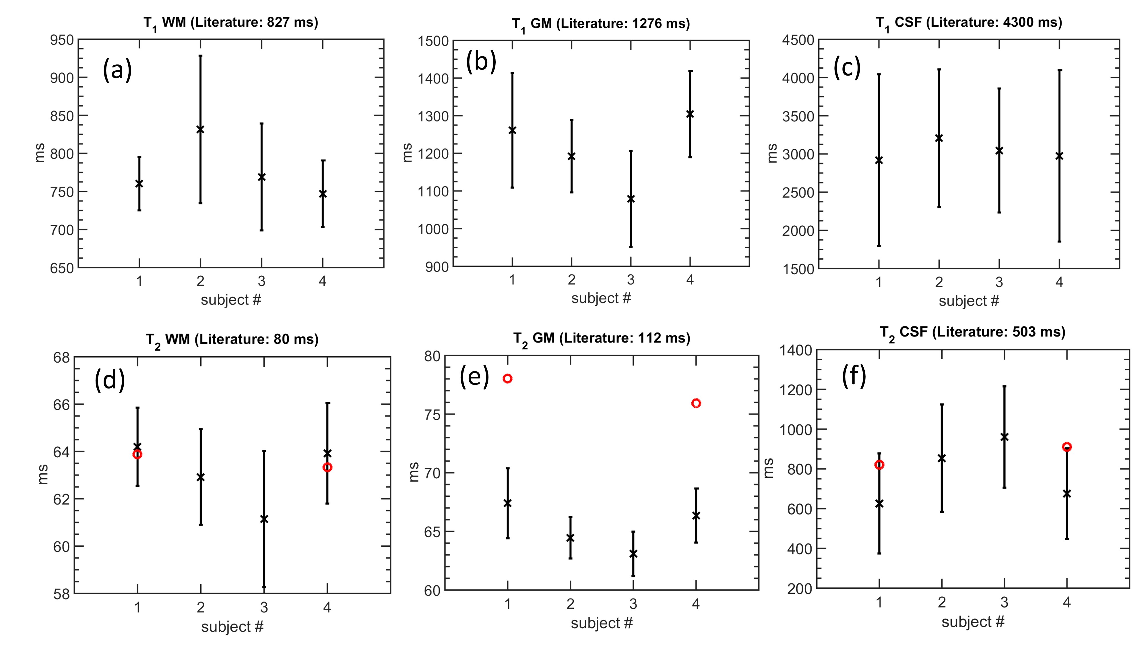
NAA distributions quantified using WAQ-MRF, $$$[NAA]_{MRF}$$$, show qualitative agreement with distributions $$$[NAA]_{SEG}$$$ calculated from segmentation and literature relaxation values (Fig. 3(a) – (c)). Similarly, distributions of $$$f_{CSF}$$$ also show qualitative agreement between the fully-relaxed acquisition, WAQ-MRF, and segmentation (Fig. 3(d)-(f)). Plots of $$$[NAA]$$$ and relaxation times as functions of grey matter volume fraction are used to estimate global values estimates of these quantities that are consistent with literature values (Figs. 4 and 5).

Discussion

Values of relaxation times, CSF mole fractions, and metabolite distributions measured with WAQ-MRF are approximately consistent with those obtained using standard methods. Measured $$$T_2$$$ relaxation times in GM are lower for WAQ-MRF than for the fully-relaxed case, likely indicating underestimation of $$$T_2$$$ in GM by WAQ-MRF. It is possible that sensitivity of the WAQ-MRF sequence to differences in $$$T_2$$$ values between GM and WM could be improved by including more TE values in the range of 60 ms to 120 ms, where the $$$T_2$$$ differences between these tissue types will be most pronounced.

Conclusion

WAQ-MRF provides subject-specific corrections of partial volume and relaxation effects for water-scaled data. By adding a one minute scan to a standard MRSI acquisition it is possible to eliminate the need for assuming literature values of relaxation and proton density to correct the water signal. We expect that the elimination of these assumptions will improve the accuracy of MRSI quantification.

Acknowledgements

This work was funded by Abbott Nutrition through the Center for Nutrition, Learning, and Memory at the University of Illinois at Urbana-Champaign.

We thank Nancy Dodge and Holly Tracy for assistance in performing the experiments.

References

1. Ma, D., et al., Magnetic resonance fingerprinting. Nature, 2013. 495(7440): p. 187-192.

2. Gasparovic, C., et al., Use of tissue water as a concentration reference for proton spectroscopic imaging. Magnetic Resonance in Medicine, 2006. 55(6): p. 1219-1226.

3. Wansapura, J.P., et al., NMR relaxation times in the human brain at 3.0 tesla. Jmri-Journal of Magnetic Resonance Imaging, 1999. 9(4): p. 531-538.

4. Rooney, W.D., et al., Magnetic field and tissue dependencies of human brain longitudinal (H2O)-H-1 relaxation in vivo. Magnetic Resonance in Medicine, 2007. 57(2): p. 308-318.

5. Piechnik, S.K., et al., Functional Changes in CSF Volume Estimated Using Measurement of Water T(2) Relaxation. Magnetic Resonance in Medicine, 2009. 61(3): p. 579-586.

6. Gutteridge, S., C. Ramanathan, and R. Bowtell, Mapping the absolute value of M-0 using dipolar field effects. Magnetic Resonance in Medicine, 2002. 47(5): p. 871-879.

7. Ernst, T., R. Kreis, and B.D. Ross, Absolute Quantitation of Water and Metabolites in the Human Brain .1. Compartments and Water. Journal of Magnetic Resonance Series B, 1993. 102(1): p. 1-8. 8. Mlynarik, V., S. Gruber, and E. Moser, Proton T-1 and T-2 relaxation times of human brain metabolites at 3 Tesla. Nmr in Biomedicine, 2001. 14(5): p. 325-331.

Figures

Fig. 1 Placement of single-slice used for WAQ-MRF and MRSI measurements.

Fig. 2 (a) Black diamonds and black solid lines show measurements of water signal for each repetition for one of the WAQ-MRF sequences. Red circles and red dashed lines show fits to the data obtained with Bloch simulations. (b) Fully relaxed (TR = 20 s) data, used to measure T2 in brain and CSF, and CSF mole fraction in the same voxel shown in (a). This is done by first fitting a single exponential to CSF data at TE > 900 ms, and then subtracting extrapolated CSF signal at TE < 150 ms to fit relaxation of brain water.

Fig. 3 (a) Structural image of middle 6 x 6 voxels used for metabolite quantification. (b) – (c) Distribution maps of (b) $$$[NAA]_{SEG}$$$ and (c) $$$[NAA]_{MRF}$$$. For $$$[NAA]_{SEG}$$$, literature proton density values are 0.78 (GM) and 0.70 (WM), and literature relaxation times are given in Fig. 5. For both $$$[NAA]_{MRF}$$$ and $$$[NAA]_{SEG}$$$, NAA relaxation is taken to be mean of GM and WM values from the literature (T1 = 1410 ms, T2 = 271 ms) [8]. (d) –(f) Maps of CSF mole fraction obtained from (d) fully-relaxed acquisition (e) segmentation, corrected for the point spread function of the double phase-encoded MRSI acquisition, and (f) WAQ-MRF.

Fig. 4 [NAA] and relaxation times as functions of the mole fraction of grey matter water $$$\phi_{GM}= f_{GM}/(f_{GM}+f_{WM})$$$, estimated from segmentation and corrected for the point spread function of the MRSI scan. Symbols denote mean values, and bars denote standard deviations of the seven WAQ-MRF scans. Linear plots are used to estimate global values at WM ($$$\phi_{GM}= 0$$$) and GM ($$$\phi_{GM}= 1$$$). (a) $$$[NAA]_{MRF}$$$ (black) and $$$[NAA]_{SEG}$$$ (blue) (b) $$$T_1$$$ from WAQ-MRF (c) $$$T_2$$$ from WAQ-MRF (black) and from fully relaxed acquisitions (red). (d) Reproduction of (a), except $$$[NAA]_{SEG}$$$ is calculated using subject-specific global values of $$$T_1$$$ and $$$T_2$$$ in GM and WM.

Fig. 5 Global estimates of $$$T_1$$$ and $$$T_2$$$ variation in measured parameters across four subjects. Black x symbols denote mean values and bars denote standard deviations from the seven MRF scans. Red circles denote $$$T_2$$$ values measured from the fully relaxed acquisition.

Proc. Intl. Soc. Mag. Reson. Med. 26 (2018)

1323