Synopsis

We propose a new methodology to denoise MRS spectrum with a focus on the acquisition time diminution. Using a discrete orthogonal polynomials, we detect two types of areas : homogenous and non-homogenous (metabolite peaks). Once these areas detected, we compute the Noise Level Function (NLF). Then, using the NLF, we use orthogonal polynomials to reconstruct a signal with a strategy for each type of area. As results, a denoising method is provided and it helps to correct the noise due to the acquisition time diminution with a good metabolite peaks conservation.

Introduction

Nowadays, MRS (Magnetic Resonance Spectroscopy) is a useful tool for diagnosis. In case of brain tumor, especially glioma, it helps to predict the tumor's evolution in the WHO classification¹ with a specific spectroscopic follow-up². In order to accelerate the whole protocol, the spectroscopy acquisition time needs to be reduced. To reduce it, the quality assessement needs to be perfomed to evaluate the usability of the spectrum for a diagnostic purpose. Consequently, we propose a new denoising method of the raw data based on orthogonal polynomials. This new data post processing aims to decrease the acquisition time without modifying metabolite concentrations.

Methods

From the original work of Sutour et al.³, the spectrum denoising is following several crucial steps: homogeneous area detection, Noise Level Function (NLF) calculation and denoising. The NLF is a function which describe the noise within a spectrum. This function is estimated using mean ($$$\mu$$$) and variance ($$$\sigma^2$$$) computed from each homogeneous region.

$$ \sigma^2 = \text{NLF}(\mu) = {a\mu}^2+b\mu+c $$

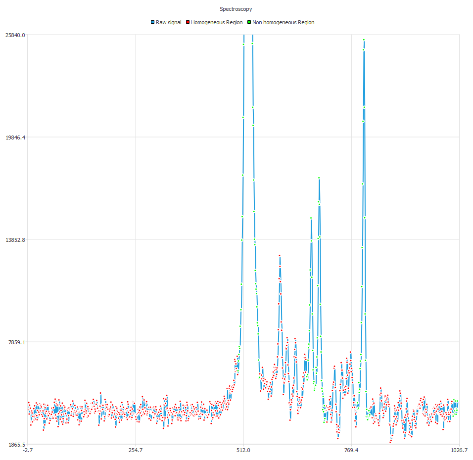
In order to complete all these steps, an application was designed and use the SLIP library⁴ to process all data. The homogeneous areas (Figure 1) are detected using a the projection coefficients of sliding localized blocks $$$W(x-kT)$$$ of the spectrum signal $$$S(x)$$$ onto the base of Legendre discrete orthogonal polynomials. The polynomials are computed using the three terms recurrence :

$$S(x)W(x-kT) = \sum_{n=0}^N a_nL_n(x)$$

with T the period of localized blocks, $$$k \in \mathbb{N}$$$ and :

$$ \left\{ \begin{array}{lcc} L_{-1}(x) &=& 0, \forall x \in I\\ L_0(x) &=& 1\\ (n+1)L_{n+1}(x) &=& (2n+1)xL_n(x) + n L_{n-1}(x)\, n \ge 1 \\ \end{array} \right. $$

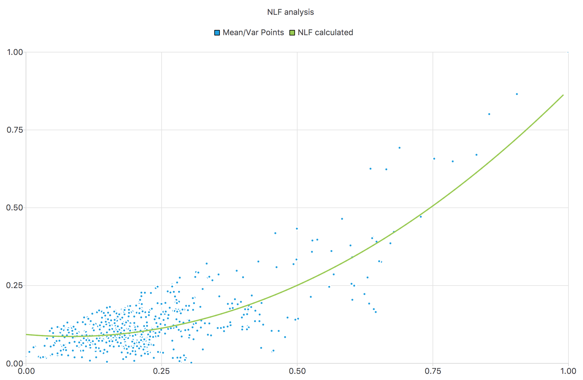
Computing the energy $$$\mathcal{E}$$$ of the localized block and projection coefficients, we can detect if the block is homogeneous or not and get the mean and variance of each block. Moreover, to preserve important metabolite peaks, masks were designed to preserve them in the analysis part. From this, we can compute the NLF using Iterative Reweighted Least Squares⁵ which is representing the spectrum's noise (Figure 2). Once the block detected, two types are defined: homogeneous and non homogeneous. Two post-processings are available for these areas. The first one, for homogeneous areas, is projection on a the same basis as the region's detection. Then, the signal is reconstructed using the first term of the coefficient found ($$$a_0$$$). For the second category, the denoising part is different. We also project on the orthogonal basis but we reconstruct the signal with the most adaptated number of coefficients:

$$ \min_{i \in \left\lbrace 0, N \right\rbrace} \left\lbrace \mathcal{E} - \sigma^{2} \leq \sum \limits_{k=0}^i a_k^2 \right\rbrace$$

To test our algorithm, we use synthetic data created within the Vespa Suite⁶. We calculated NLF on real data and applied the detected noise on our synthetic data to simulate in vivo noise regarding the number of excitations.

Results

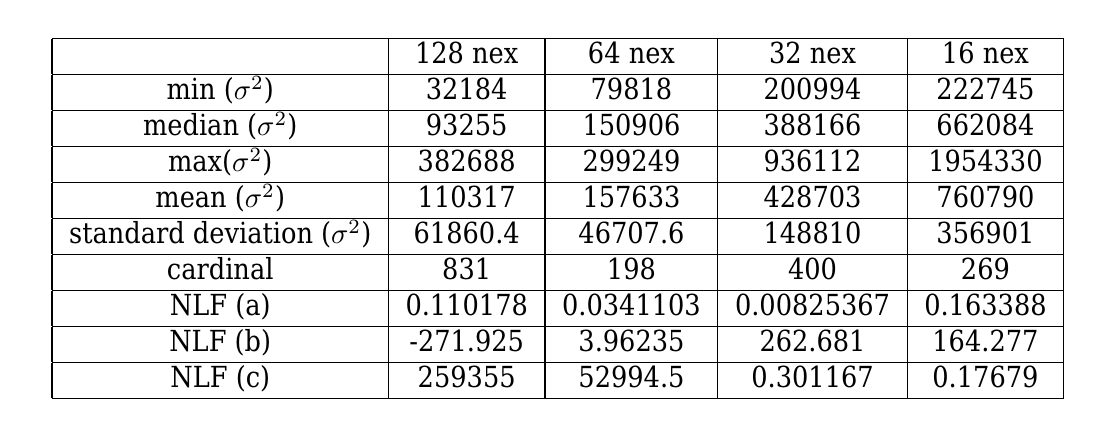
NLF were calculated for several sequences from 16 to 128 excitations (Nex) on a Skyra 3T (Siemens Healthineers, Erlangen, Germany) with an acquisition time from 30 secondes to 4:00 min. The sequence PRESS SVS parameters are the following : TE = 135ms, TR = 1300ms, 1024 FID points with a 15x15x15mm voxel size. First, noise caracterization is the first step to adapt the denoisig strategy to our data. On our current dataset, we compute several statistics regarding the number of excitations (Figure 3).

It gives us important informations about the distributions of the variance values within the homogenous areas. Then, the NLF is computed and gives informations regarding the type of noise. From Sutour et al.³ a constant NLF is typical of an additive noise such as Gaussian noise. A linear NLF is typical of a multiplicative noise and a parabolic NLF represents noise mixture, Gaussian and multiplication noise for example. The noise level function estimated on our data is mostly computed as a parabolic function.

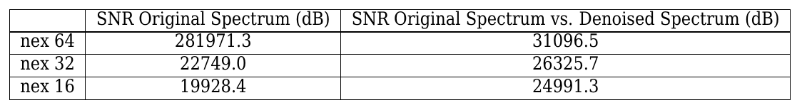
In order to evaluate our denoising, the SNR was calculated :$$ SNR_{dB} = 10 \log_{10} \frac{||S_{ref}||^2}{||S_{ref} - S||^2} $$

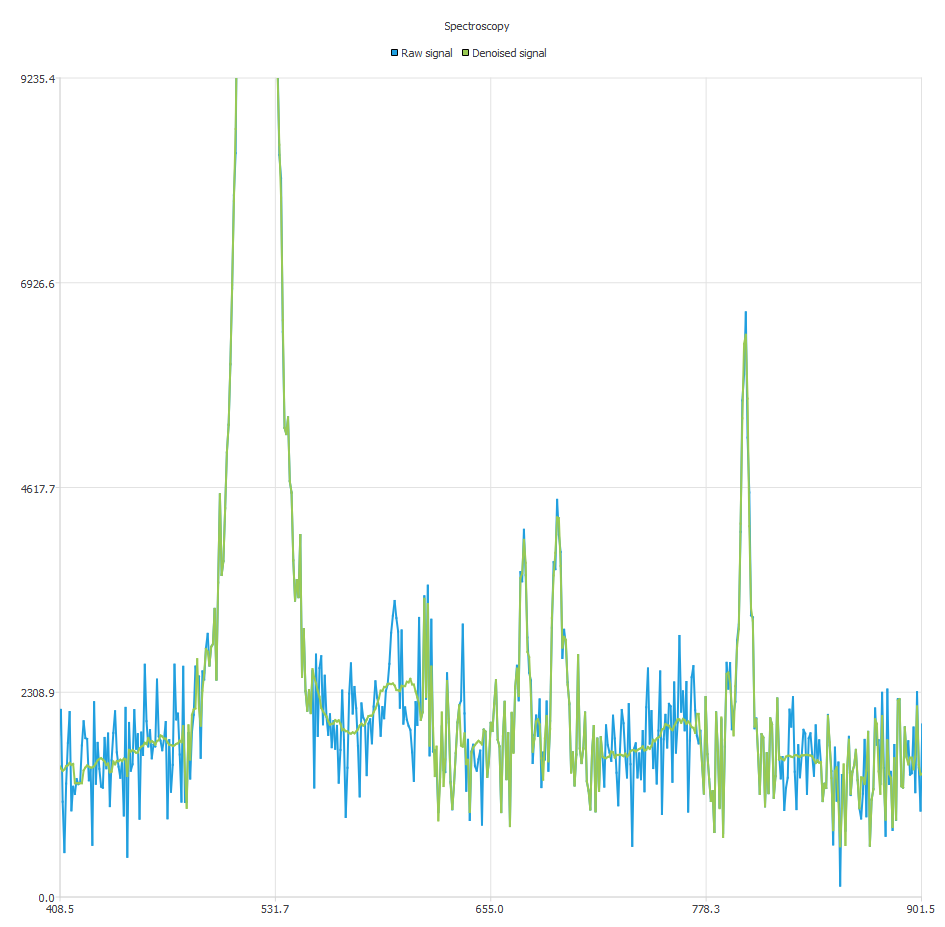
In Figure 4, our denoising shows interessing results regarding the SNR calculated with the Nex = 128 spectrum as reference. In Figure 5, the denoised spectrum fits Cho, Cr and NAA peaks very well even in noisy data. The masking step and the orthogonal polynomials preserve peaks using a higher number of coefficient for the reconstruction.

Conclusion

Acknowledgements

References

[1] David N Louis, Hiroko Ohgaki, Otmar DWiestler,Webster K Cavenee, Peter C Burger, AnneJouvet, Bernd W Scheithauer, and Paul Kleihues. The 2007 who classification of tumoursof the central nervous system. Acta neuropathologica, 114(2):97–109, 2007.

[2] Rémy Guillevin, Carole Menuel, Jean-Noël Vallée, Jean-Pierre Françoise, Laurent Capelle,Christophe Habas, Giovanni De Marco, Jacques Chiras, and Robert Costalat. Mathematicalmodeling of energy metabolism and hemodynamics of who grade ii gliomas using in vivomr data. Comptes rendus biologies, 334(1):31–38, 2011.

[3] Camille Sutour, Charles-Alban Deledalle, and Jean-François Aujol. Estimation of the noiselevel function based on a nonparametric detection of homogeneous image regions. SIAMJournal on Imaging Sciences, 8(4):2622–2661, 2015.

[4] Benoit Tremblais, Laurent David, Denis Arrivault, Julien Dombre, Lionel Thomas, and LudovicChatellier. Simple library of image processing (slip). 2010.

[5] Peter J Green. Iteratively reweighted least squares for maximum likelihood estimation,and some robust and resistant alternatives. Journal of the Royal Statistical Society. SeriesB (Methodological), pages 149–192, 1984.

[6] Vespa suite (versatile simulation, pulses and analysis). https://scion.duhs.duke.edu/vespa/. Accessed: 2017-05-22.