1319

Novel methodology for processing, quality assessment, and artifact mitigation of raw 2D Correlation Spectroscopy data

Laura J Mariano¹, Marcia Sahaya Louis², Benjamin Rowland³, Huijun Liao⁴, Kristin Heaton⁵, John Irvine¹, and Alexander P Lin^3,6

¹The Charles Stark Draper Laboratory, Inc., Cambridge, MA, United States, ²Electrical and Computer Engineering, Boston University, Boston, MA, United States, ³Center for Clinical Spectroscopy, Brigham and Women's Hospital, Boston, MA, United States, ⁴Psychiatric Neuroimaging Laboratory, Brigham and Women's Hospital, Boston, MA, United States, ⁵US Army Institute of Environmental Medicine, Natick, MA, United States, ⁶Harvard Medical Institute, Boston, MA, United States

Synopsis

2D Correlation Spectroscopy (COSY) can be used to identify and study coupled resonances that cannot be observed or distinguished in 1D NMR spectra. However, resources and literature on best practices for processing raw 2D COSY data are limited. In this work, we describe a novel pipeline of signal processing algorithms and visualizations for quality assessment and artifact mitigation designed specifically for raw 2D COSY data, including detection of residual H2O and lipid contamination, correction for drift across averages, and peak location correction to enable more accurate comparisons of metabolites across subjects.

Introduction

2D Correlation Spectroscopy (COSY) can be used to identify and study coupled resonances that cannot be observed or distinguished in 1D NMR spectra¹. However, the increased information it provides also increases the complexity of the methods required to extract high quality 2D spectra from raw scanner data, and the literature on best practices for signal processing and quality assessment in 2D COSY data is limited. To address these issues, we have developed a suite of Python-based signal processing algorithms and visualizations for quality assessment and artifact mitigation designed specifically for 2D COSY data. These methods include detection of residual H2O and lipid contamination, correction for drift across averages, and peak location correction to enable more accurate comparisons of metabolites across subjects.

2D COSY pre-processing

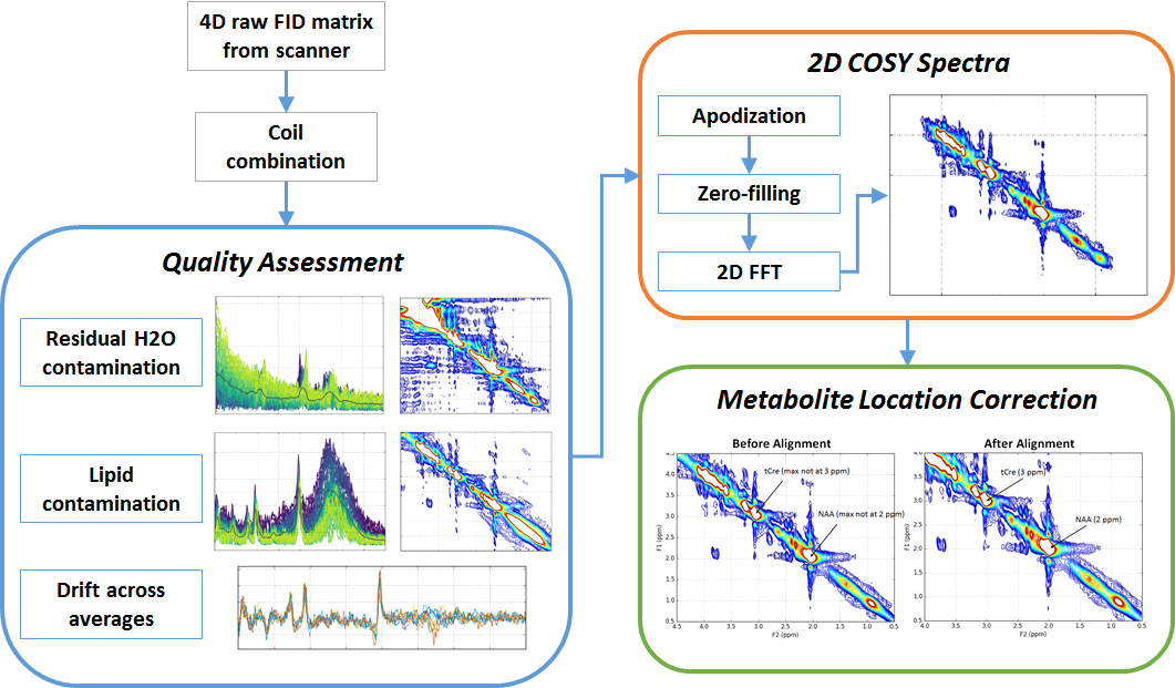
Figure 1 depicts the 2D COSY processing pipeline, which starts with raw scanner data containing the free induction decay (FID) signal acquired from each coil for each t1 increment, often with multiple repeated acquisitions (averages) for each of the increments. This creates a 4-dimensional complex matrix with dimensions [t1 increments x samples x averages x coils]. The dataset used in the following example was collected from a Siemens 3T scanner (TIM Skyra, VD11) using a 32 channel head coil. 2D COSY was acquired with a starting echo time of 30 ms followed by 64 t1 increments of 0.8 ms each, 8 averages per increment, and 2048 data points². An SVD-based algorithm³ is used to derive coil weightings from the raw scanner data, which are applied to each average and t1 increment, creating a [64 x 2048 x 8] matrix.

2D COSY signal quality assessment

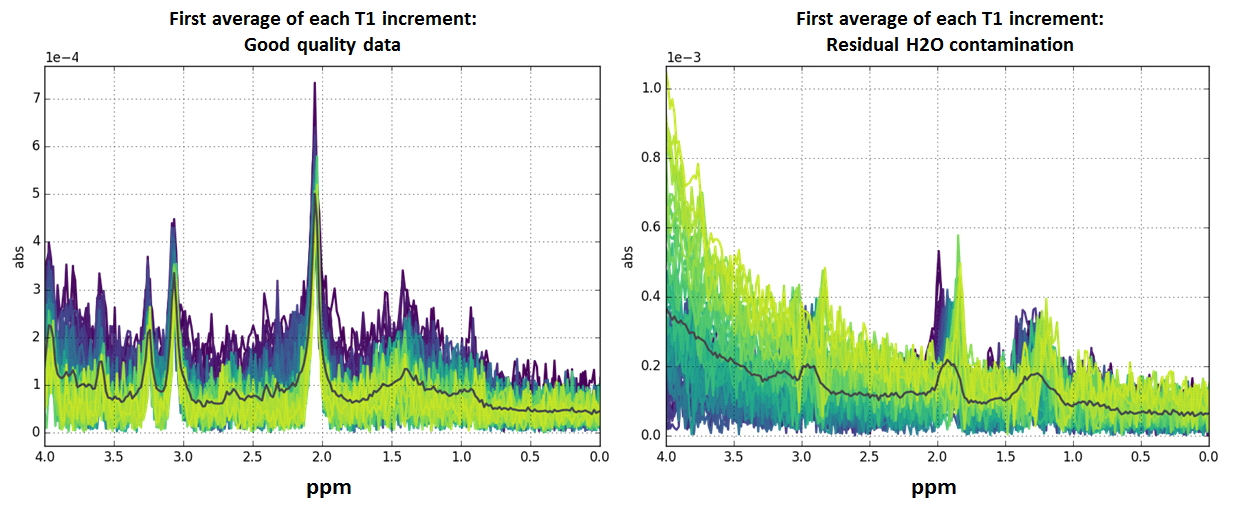
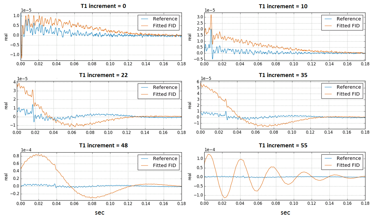
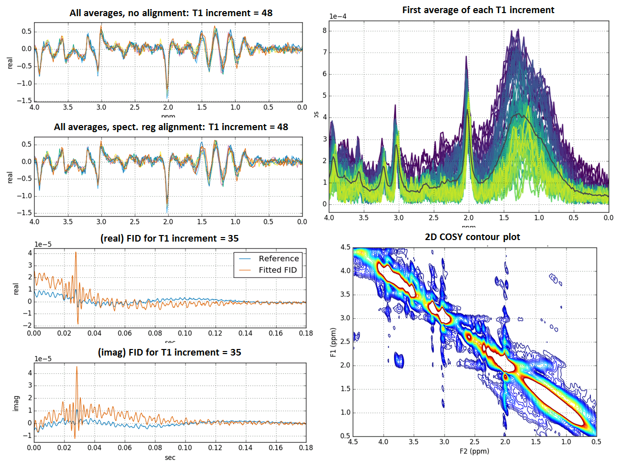
At this stage in the processing pipeline, failure of H2O suppression, lipid contamination, and issues with signal drift across averages can generally be detected visually, so we developed a series of simple diagnostic visualizations designed to rapidly highlight these kinds of issues. Contamination of the metabolite region of the spectrum by residual H2O changes the magnitude and shape of the signals in characteristic ways in the time and frequency domains⁴. It can begin at any point in the scan, thus affecting some increments and not others. Figures 2 and 3 depict diagnostic visualizations designed to highlight if and when issues with the H2O suppression process developed during the acquisition. These same views of the data can also be used to spot lipid contamination, as shown in Figure 4, and reveal issues with signal drift across averages. If drift is detected, it is fixed at this point using an implementation of the spectral registration algorithm⁵.

Generating the 2D COSY spectra and metabolite location correction

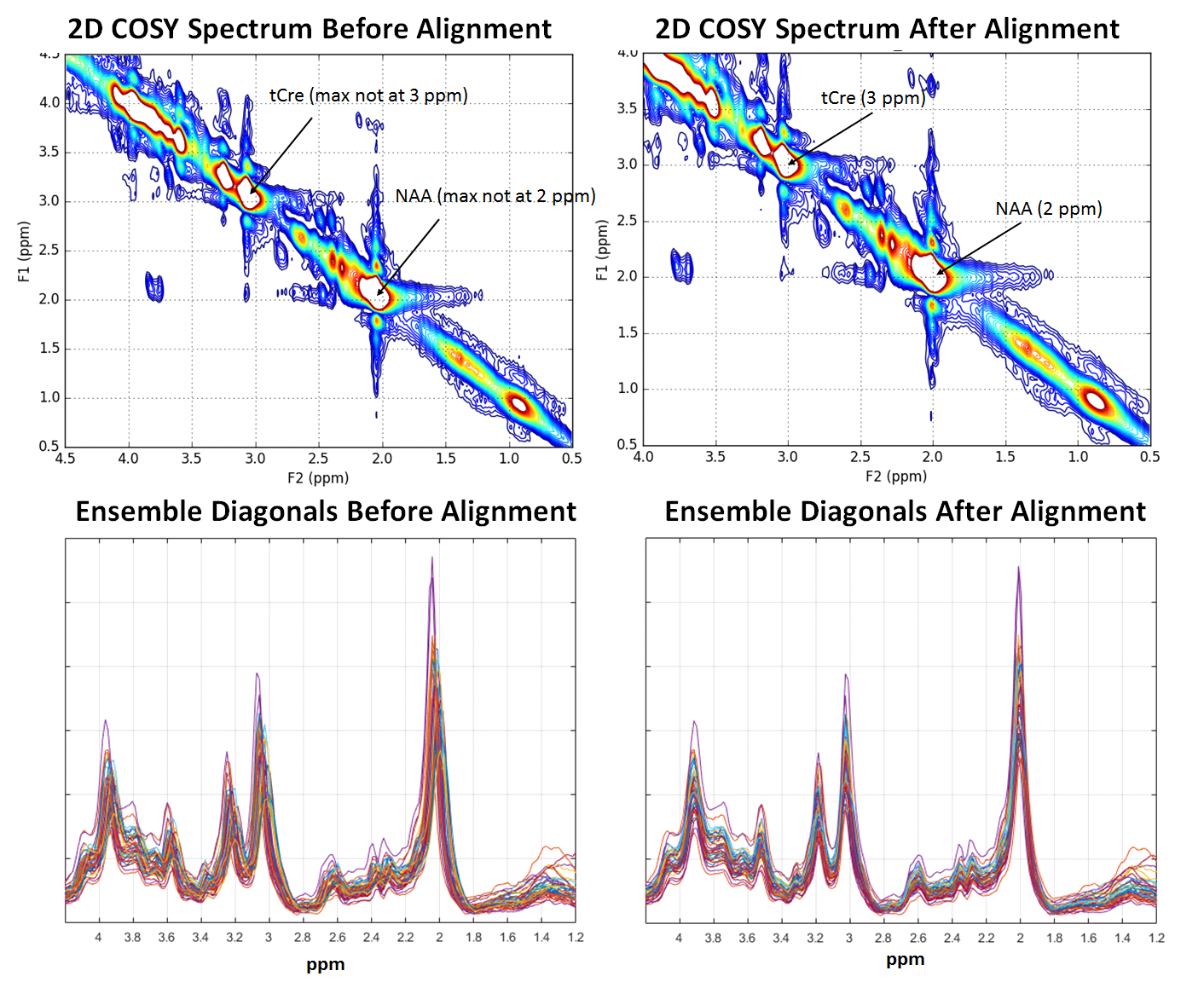
After coil weighting, quality assessment and correction for signal drift, we average the averages, apply apodization using a Tukey window, zero-fill the FIDs to increase the f1 frequency domain resolution, and perform a 2D Fast Fourier Transform. At this point, metabolite quantification can be performed; however, we’ve observed many cases where major metabolite peaks such as N-acetylaspartate (NAA) and Creatine are offset from their correct locations in the 2D parts-per-million (ppm) plane, as shown in Figure 5, top. These offsets are not necessarily the same for all individuals, making it difficult to compare metabolites across a population of subjects. To solve this problem, we developed a metabolite location correction algorithm designed to adjust peak locations, but not alter their amplitudes. We first extract the values that lay as close to the diagonal as possible in the 2D COSY matrix, and identify peak locations (in Hz) in the diagonal signal that are closest to a set of landmark singlets: N-acetylaspartate (2.008 ppm), Creatine (3.027 and 3.913 ppm), Choline (3.185 ppm), and myo-inositol (3.5217 ppm), for this dataset. In f1 and f2, we create a ppm axis piecewise between each pair of landmarks by finding the equation of the line intersecting the theoretical peak locations (in ppm) and the empirical peak locations (in Hz), creating a unique ppm mesh that maps the empirical peak locations to the theoretical ones. This mesh is then aligned to a common, uniformly sampled reference ppm mesh using 2D interpolation. Figure 5 (bottom) illustrates the effects of the processing pipeline for an ensemble of subjects.

Conclusions

While there are toolboxes available for analysis and quantification of 2D COSY data, to our knowledge, there are few resources designed specifically for processing, quality assessment, and artifact mitigation of raw 2D COSY data. The pipeline described above provides a simple, semi-automated pre-processing approach we hope will enable more in-depth, accurate analysis of this information-rich data source.

Acknowledgements

This study was funded by the Department of Defense Congressionally Directed Medical Research Program WX81-XWH-10-1-0835. The views expressed in this abstract are those of the authors and do not reflect the official policy of the Department of Army, Department of Defense, or the U.S. Government.

References

1. Thomas, M.A., et al., Localized two‐dimensional shift correlated MR spectroscopy of human brain. Magnetic Resonance in Medicine, 2001. 46(1): p. 58-67.

2. Lin, A.P., et al., Changes in the neurochemistry of athletes with repetitive brain trauma: preliminary results using localized correlated spectroscopy. Alzheimer's research & therapy, 2015. 7(1): p. 13.

3. Rodgers, C.T. and M.D. Robson, Receive array magnetic resonance spectroscopy: whitened singular value decomposition (WSVD) gives optimal Bayesian solution. Magnetic Resonance in Medicine, 2010. 63(4): p. 881-891.

4. Kreis, R., Issues of spectral quality in clinical 1H‐magnetic resonance spectroscopy and a gallery of artifacts. NMR in Biomedicine, 2004. 17(6): p. 361-381.

5. Near, J., et al., Frequency and phase drift correction of magnetic resonance spectroscopy data by spectral registration in the time domain. Magnetic Resonance in Medicine, 2015. 73(1): p. 44-50.

Figures

Figure 1: The 2D COSY processing pipeline converts raw, unprocessed FIDs into 2D spectra that can be used for quantification of metabolite concentrations. After coil combination, a quality assessment phase generates diagnostic visualizations designed to highlight issues with residual H2O and lipid contamination, and drift across averages. The FIDs are then apodized, zero-filled, and converted to the frequency domain using a 2D FFT. Finally, metabolite peak locations are corrected through alignment with a set of singlet landmarks with known locations in the 2D ppm plane.

Figure 2: Frequency-domain representations of the change in overall signal magnitude as the COSY scan progresses over time (over t1 increments). Each axis contains plots of the spectrum of the first average (of 8) for each t1 increment overlaid on top of each other. The color of the line corresponds to the t1 increment, going from purple (first) to light green (last). On the left is an example of a good quality dataset, and on the right is an example where the residual H2O signal drifts into the metabolite region as the t1 increments progress in time.

Figure 3: A time-domain (FID) view of a 2D COSY acquisition that developed issues with H2O suppression as the scans progressed. Each axis corresponds to a different t1 increment (0, 10, 22, 35, 48, 55). The FID for the test subject is plotted in red, and in blue is the FID of a reference subject with good quality data for the same t1 increment. The test subject’s data has been temporally aligned with the reference subject for comparison purposes.

Figure 4: Four visualizations depicting characteristics of lipid contamination. Upper left: All averages for increment 48 show a high frequency oscillation in the 1.0-1.5 ppm range. Upper right: The first average of each increment has a significant increase in signal magnitude in the 1.0-1.5 ppm region. Bottom left: The FID of the 35^th increment contains high frequency oscillations. Bottom right: A long, broad peak in the 2D contour plot in the 1.0-1.5 ppm region indicates lipid contamination.

Figure 5: (Top) 2D COSY spectra before and after metabolite location correction. On the left, two of the largest single peaks, NAA and tCre are offset from their theoretical locations on the diagonal of the matrix. On the right, after adjustment, these singlets lie much closer to their correct locations. (Bottom) Overlays of the diagonals of the 2D COSY matrices of an ensemble of subjects before (left) and after (right) metabolite peak adjustment. Before correction, alignment across subjects is poor which will make it difficult to compare metabolites. After, the major peaks on the diagonal are much better aligned.

Proc. Intl. Soc. Mag. Reson. Med. 26 (2018)

1319