1314
Toward Absolute Quantification Using External Reference Standards at 3T and 9.4T1Biological Cybernetics, Max Planck Institute, Tübingen, Germany, 2IMPRS for Cognitive and Systems Neuroscience, Eberhard-Karls University of Tübingen, Tübingen, Germany, 3Institute of Physics, Ernst-Moritz-Arndt University Greifswald, Greifswald, Germany
Synopsis
Absolute quantification is a challenge with many paths to reach the final goal of quantifying metabolites in absolute units (e.g. Molarity and molality). Utilizing an external reference standard (ERF) is an attractive method for quantifying in vivo metabolites due to the ability for direct comparison between a known concentration of a metabolite and the in vivo data. A major concern in utilization of an ERF is the differences in coil loading between in vivo and in vitro measurements. To that end, this work describes a method to calibrate and adjust the transmitter voltage in order to maximize signal detection independently of coil load.
Introduction
Quantification of cerebral metabolites in absolute units (e.g. Molarity and molality) is a vital attribute in accurate classification of neurological diseases and disorders. Many groups choose to utilize internal water referencing(IWR) for absolute quantification; however, in diseases where internal water is potentially unstable (e.g. Multiple Sclerosis1 or tumors) internal water referencing is unlikely to yield accurate quantification. External reference standards (ERF) with coil loading correction based on the principle of reciprocity2,3 (POR) has shown reliable quantification results at 3T4-6. A reliable localized power optimization method crucial for this quantification strategy was implemented. In this work, toward absolute quantification using ERF for human brain MRS application at 9.4T, a method was developed for tip angle optimization based on B1 mapping for accurate localized transmitter voltage adjustment.Methods
B1-mapping was utilized to observe the tip angles achieved in a localized 2x2x2cm3 voxel in-vitro at both 3T and 9.4T. A transmitter voltage correction was applied based on the tip angle achieved such that:
Vcorrected = (θtarget/θmeasured) x Vnominal.
Where Vnominal was selected as 250V at 9.4T and 220V at 3T for all scans and was selected as 90° for 9.4T and 8° at 3T. A STEAM sequence was utilized at 3T (TE/TM/TR = 20/10/4000 ms) and 9.4T (TE/TM/TR = 11/50/5000 ms) without and with water suppression for analysis of the water and NAA signals respectively. A comparison of B1-mapping sequences (TurboFLASH and AFI6) was performed to compare the accuracy of the measured flip angle for each B1 mapping sequence as input to calculate Vcorrected.
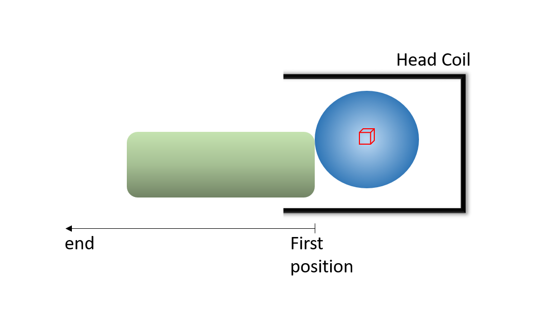
The designed coil loading scheme (Fig. 1) for testing the reliability of the method involved using two phantoms in similar manners at both field strengths. A spectroscopy phantom was placed securely in the head coil and was used to measure in the isocenter of the phantom while a large tube phantom (Fig. 1) was used to load the coil incrementally. The tube phantom was placed immediately at the foot of the spectroscopy phantom and incrementally adjusted away from the spectroscopy phantom, in the foot-direction, by 1cm. At 3T a 64-channel receive-only birdcage head coil was used for signal detection and the body coil was used as the transmitter. At 9.4T a homebuilt T/R phased-array head coil was used as transmitter and receiver7. At each loading position Siemens 2nd-order shimming was applied for both field strengths. MATLAB was used for reconstruction of data and statistical tests were performed using R (3.4.2).
Results
Based on the water signal detected following the B1 mapping voltage adjustment, TurboFLASH yielded the more accurate flip angle optimization in comparison to AFI-mapping. This effect is seen in Fig. 2 where the water signal increased for TurboFLASH when comparing Vnominal and Vadjusted; whereas, the signal decreased when using AFI for calculation of Vadjusted. Adjustment of the transmitter voltage based on TurboFlash B1+ mapping allowed for increased signal detection at both 3T and 9.4T across a variety of coil loads. The voltage correction method applied with TurboFLASH increased the water signal by an average percent change of 17.5%±4.8% at 9.4T (Fig. 3) and 9.9%±0.1% at 3T (Fig. 4).
The range of the applied correction factor is relatively small; with the applied voltages ranging from 197.7-199.2V at 3T and 185.4-205.6V at 9.4T when loaded with both the spectroscopy phantom and tube phantom. NAA/water is more stable when TurboFLASH voltage correction is applied (Fig. 5). NAA/water signal is 9.9% increased when a localized transmitter voltage optimization is applied compared to when the nominal voltage is used for acquisition.
Discussion
It is evident from work at both 3T and 9.4T that using suboptimal transmit voltages results in severe signal loss. In this case, using the AFI sequence showed not to be optimal for accurate localized voltage adjustment due to its limited dynamic range especially in case of strong B1+ inhogeneity at 9.4T. TurboFlash based B1+ mapping is better suited for accurate flip angle estimation at ultra high fields and shall be used in the context of reciprocity based external referencing in future.Conclusion
Achieving increased signal by performing localized power optimization highlights the importance of using optimized transmitter voltages. It is likely that the optimal transmitter voltage is different for each individual due to different coil loading, and corrections for each subject allow for the detection of maximum signal when the specified tip angle is achieved. The method used in this work proves to be robust in achieving optimal flip angles for strong B1+ inhomogeneity, varying coils and coil loads thus allowing a more accurate application of transmitter voltage to achieve a desired tip angle.Acknowledgements
Funding by the European Union (ERC Starting Grant, SYNAPLAST MR, Grant Number: 679927) is gratefully acknowledged.References
- Moccia M, Ciccarelli O. Molecular and Metabolic Imaging in Multiple Sclerosis. Neuroimaging Clin N Am. 2017;27(2):343-356. doi:10.1016/j.nic.2016.12.005.
- Hoult D., Richards R. The signal-to-noise ratio of the nuclear magnetic resonance experiment. J Magn Reson. 1976;24(1):71-85. doi:10.1016/0022-2364(76)90233-X.
- Hoult DI. The principle of reciprocity in signal strength calculations?A mathematical guide. Concepts Magn Reson. 2000;12(4):173-187. doi:10.1002/1099-0534(2000)12:4<173::AID-CMR1>3.0.CO;2-Q.
- Jost G, Harting I, Heiland S. Quantitative single-voxel spectroscopy: The reciprocity principle for receive-only head coils. J Magn Reson Imaging. 2005;21(1):66-71. doi:10.1002/jmri.20236.
- Helms G. The principles of quantification applied to in vivo proton MR spectroscopy. Eur J Radiol. 2008;67(2):218-229. doi:10.1016/j.ejrad.2008.02.034.
- Yarnykh VL. Actual flip-angle imaging in the pulsed steady state: A method for rapid three-dimensional mapping of the transmitted radiofrequency field. Magn Reson Med. 2007;57(1):192-200. doi:10.1002/mrm.21120.
- Avdievich N, Giapitzakis IA, Henning A. Optimization of the receive performance of a tight-fit transceiver phased array for human brain imaging at 9.4T. In Proceedings of the 25th Annual Meeting of ISMRM, Honolulu, Hawai’i, USA, 2017. p. 25
Figures
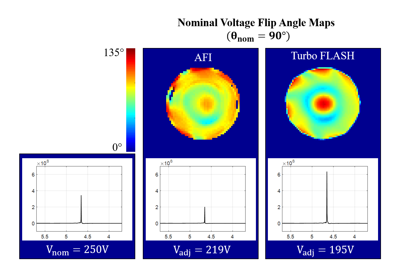
Top row: Flip angle distribution maps acquired at 9.4T once with AFI and once with the Turbo-FLASH (TFL) sequence at the nominal voltage (V=250V). The flip angle maps were used for local power optimization.
Bottom row: Unsuppressed water peaks acquired with the nominal voltage (left), with the adjusted voltage as calculated from the AFI B1+ map (middle), and with the adjusted voltage as calculated from the TFL B1+ map (middle)
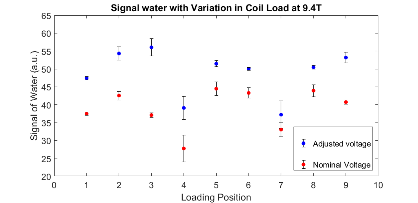
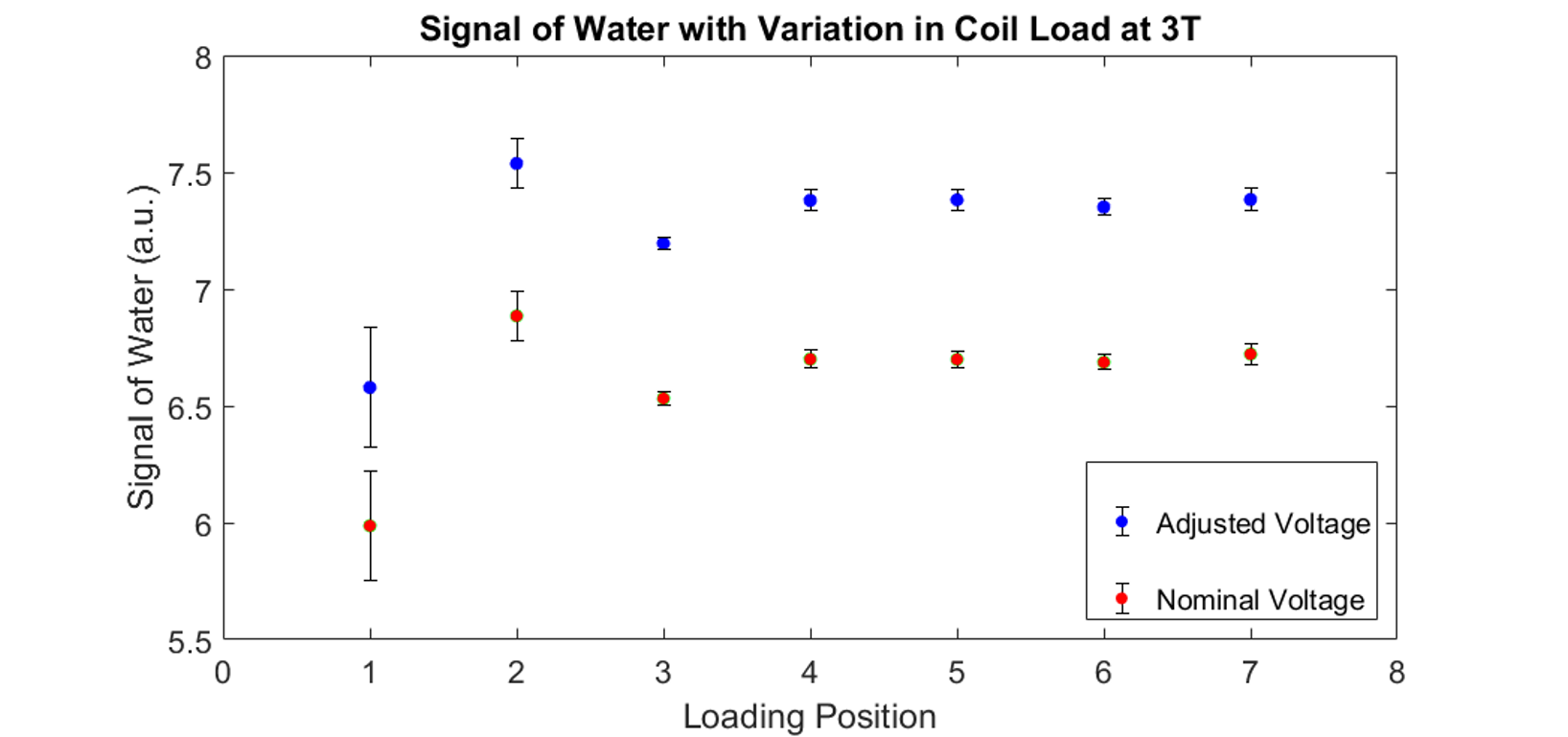
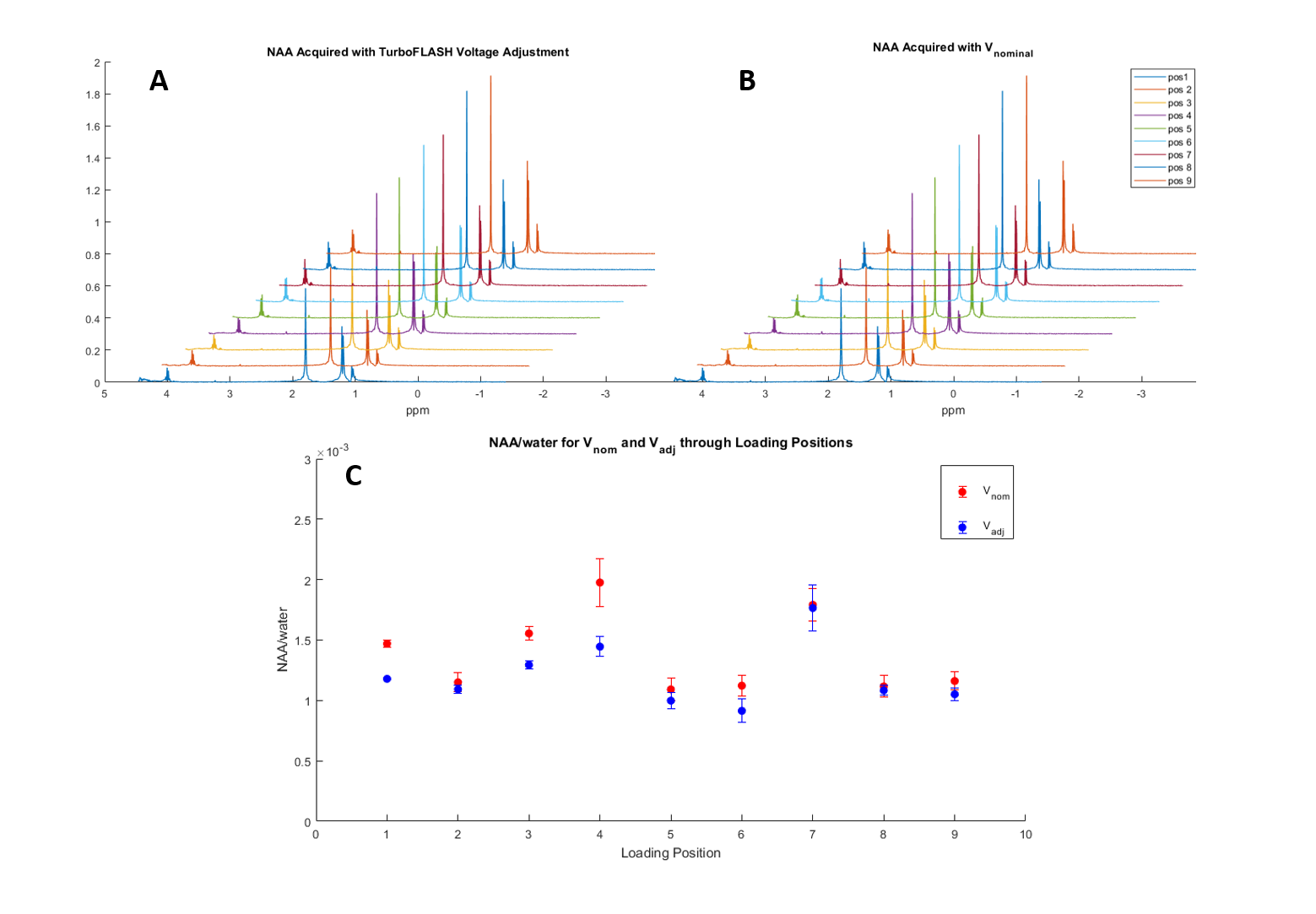
Fig. 5A: NAA/water with TurboFLASH adjusted transmitter voltage
Fig. 5B: NAA/water with the nominal transmitter voltage
Fig. 5C: Variations of NAA/water for both nominal and adjusted transmitter voltages. The smaller variation of signals acquired with Vadj is suggestive of more stable signal acquisition throughout coil loading positions.