1273
SNR and PSF Simulations for k-t Trajectories in MRSI: CSI, EPSI, Rosettes, and Concentric Rings1Weizmann Institute of Science, Rehovot, Israel
Synopsis
We compare, using numeric simulations, the point spread functions (PSF) and the SNR of different trajectories in k-t space for magnetic resonance spectral imaging (MRSI). This is a first step towards evaluating the trajectory of choice while balancing SNR efficiency, scan time, and localization of signal (resolution vs. bleed).
Introduction
Different trajectories in k-t space have been proposed over the years for magnetic resonance spectral imaging (MRSI). In choosing a trajectory, three points are of importance: the trajectory efficiency, i.e., signal-to-noise ratio (SNR) per square root of time ($$$\mathrm{SNR}/\sqrt{t}$$$); the shape of the point-spread-function (PSF), i.e., the spectrum localization and signal bleed; and the minimum needed time of acquiring a complete data set.
Three families of trajectories were simulated: Echo Planar Spectroscopic Imaging (EPSI), Rosettes,1 and a concentric rings trajectory (CRT).2 These are compared to the Chemical Shift Imaging (CSI) method.
Methods
Trajectories where designed in Matlab (Mathworks, Natick, Mass.) for typical MRSI scenarios, including low vs. high gradient systems demands, and including spectral widths (SW) appropriate for 3T and 7T systems:
- Field-of-view (FOV): 220mm.
- Desired spectral-width (SW): 1250Hz (“3T”) and 2500Hz ("7T").
- Spatial resolution: 24×24.
- Desired spectral resolution: 256.
- Hardware limitations (maximum gradient amplitude and slew rate). Set 1: Gmax = 10$$$\mathrm{\frac{mT}{m}}$$$, Smax = 60$$$\mathrm{\frac{mT}{m\cdot ms}}$$$; Set 2: Gmax = 80$$$\mathrm{\frac{mT}{m}}$$$, Smax = 200$$$\mathrm{\frac{mT}{m\cdot ms}}$$$.
- Raster times: 10$$$\mathrm{\mu s}$$$ for gradients, 2$$$\mathrm{\mu s}$$$ for acquisition dwell time, and 1$$$\mathrm{\mu s}$$$ for ADC start position.
- Trajectory types: CSI; “Standard” EPSI, acquiring on both positive and negative readout gradients (with and without ramp sampling); flyback EPSI, acquiring only on the positive readout gradients and a shortest return gradient (with and without ramp sampling); Rosettes;1 and CRT2.
The “image” $$$\hat{\rho}$$$ was reconstructed from the “measured” signal $$$S$$$ by iteratively minimizing $$\left\Vert F^{\dagger}\left(F\hat{\rho}-S\right)\right\Vert =\left\Vert \left(F^{\dagger}F\right)\hat{\rho}-\left(F^{\dagger}S\right)\right\Vert \text{, }$$ where $$$F$$$ is the (generally) non-uniform Fourier-transform from spectral image (SI) to k-t space, with $$$F^{\dagger}$$$ its adjoint. Prior to reconstruction, the signal was apodized along time. For trajectories with a disk-shape support in k-space, the reconstruction was regularized by zero-filling the corners of k-space (filling to a square). In these cases, zero k-space corners were enforced on the final results by an FFT to k-space, application of a disk shaped mask, and an inverse FFT. Noise was estimated by generating 100 noisy realization for each “experiment”. This was done for a circular disk “phantom” of diameter 100mm, at resonance, and having T*2=80ms. The same reconstruction (including apodization) was used to determine the PSFs, however for a Dirac-delta signal (at resonance) with practically infinite T*2. Sub-voxel behavior of the PSF was found by repeatedly shifting the delta function within the space-frequency “voxel” (10×10×10 sub-samples).
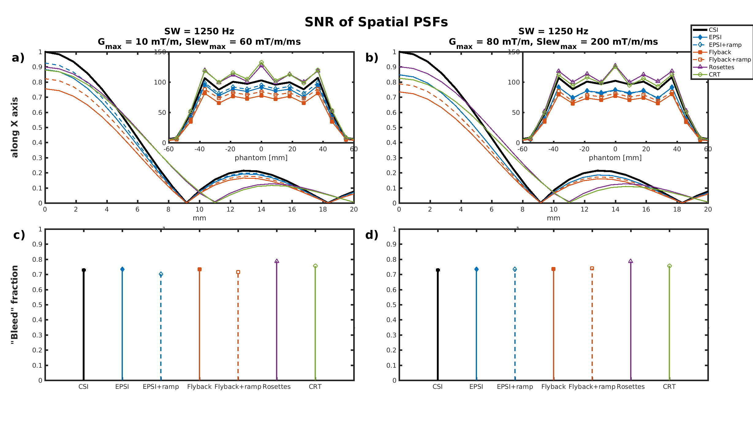
As a measure of PSF localization a 'bleed fraction' was defined: The ratio between the area under the PSF outside the central voxel/lobe to the area of the whole PSF (estimated at the xy plane, on resonance).
Results
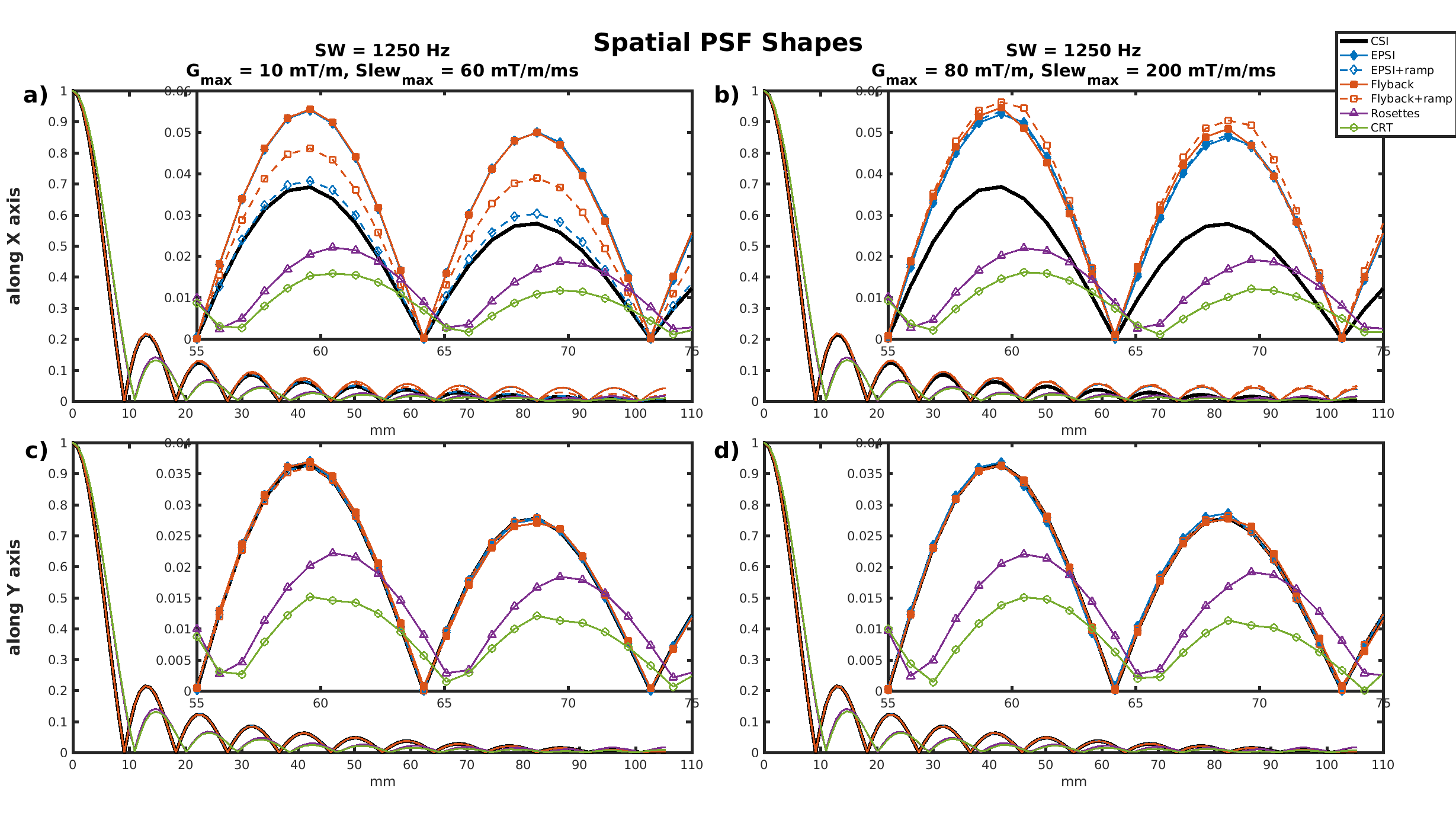
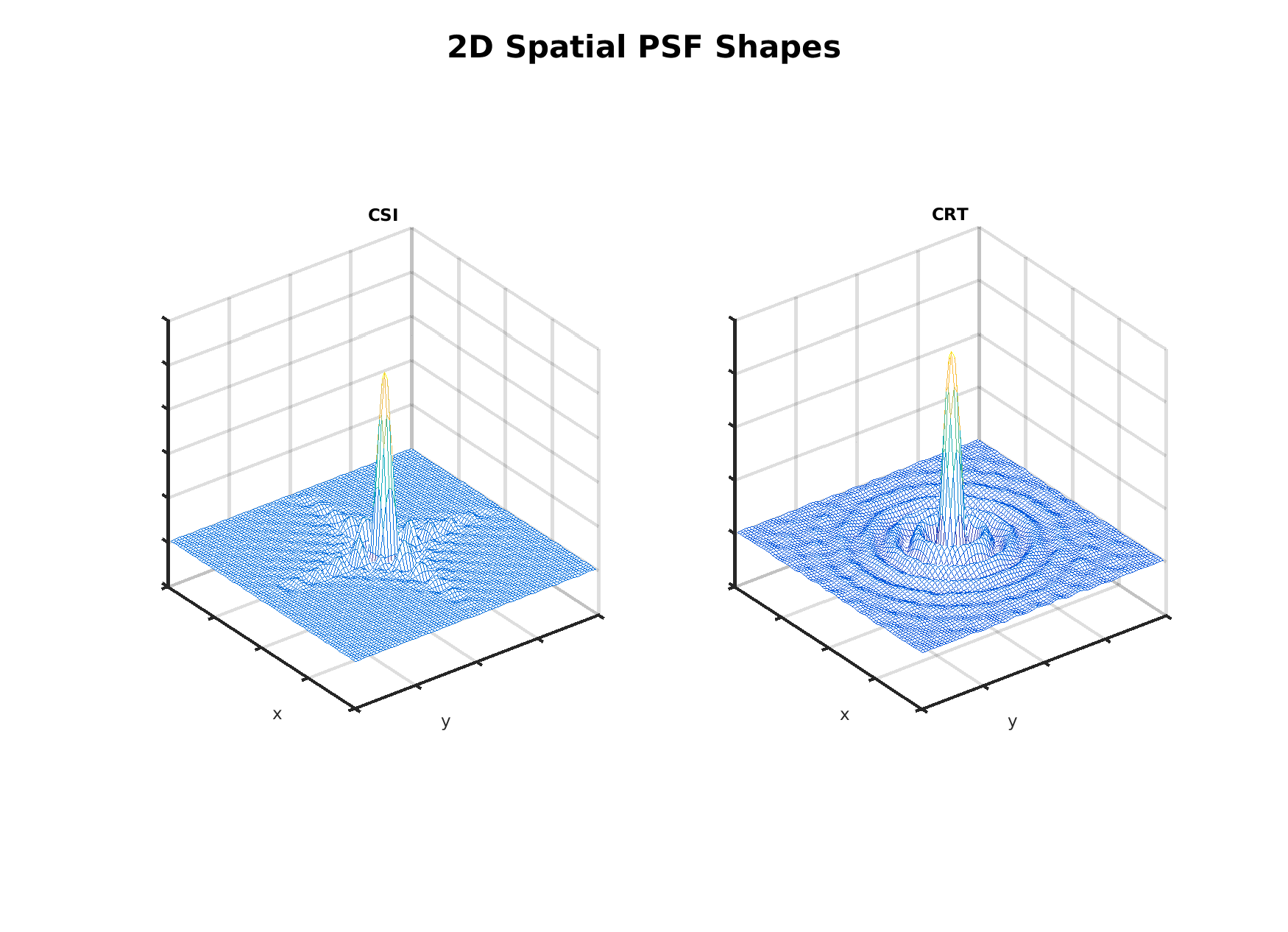
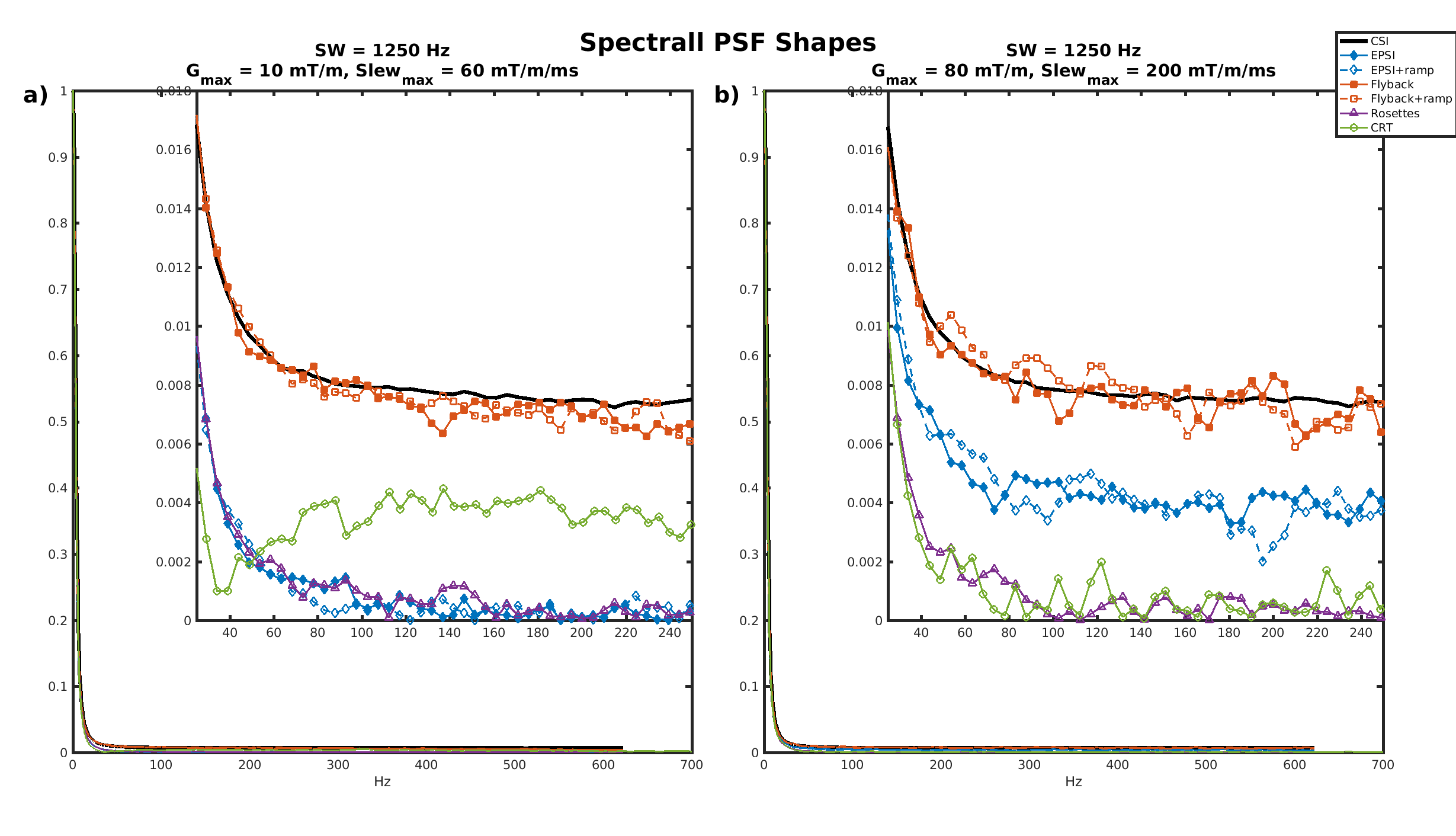
All SNR reported are normalized for comparison, accounting for different acquisition times and actual resolution/SW. Table 1 gives a summary of the SNR and bleed fraction for the cases simulated. The shapes of the spatial PSFs in two cases are shown in Fig. 1. The PSFs of the trajectories with square/disk support in k-space are markedly different, as also evident in their 2D spatial distribution in Fig. 2. Figure 3 compares SNR aspects with PSFs normalized with respect to total scan time and actual SW — the acquisition BW is treated as a trajectory “parameter” and therefore disregarded. It also shows (insets) the estimated SNR (from 100 realizations) along the center of the phantom. The bottom row depicts graphically the bleed fractions for the cases shown. Finally, Fig. 4 shows the PSF shapes along the spectral dimension for two of the cases simulated.Discussion
We attribute the most affect to the trajectory's support in k-space, i.e. disk-shape (rosettes and CRT) vs. rectangular (CSI + EPSI variations). Circular support results in a circularly symmetric PSF that effectively covers more voxels than the cross-like PSF of CSI and EPSI (Fig. 2) . The larger coverage means noise from more voxels cancels out, thus increasing the SNR simulated for CRT and Rosettes in uniform phantoms.
Ramp sampling increases SNR because acquisition time is used more efficiently, an effect more dominant at low slew rates, where the ramp time is more significant.
We found that the 'bleed fraction' does not predict SNR, presumably because it does not reflect the PSF's distribution outside the voxel.
SNR-wise, the phantom simulations should better correlate with actual brain scan, but miss localization consideration, which are of special importance when signal bleed from lipids is an issue.
For a trajectory of choice, a desired balance between SNR and localization must be defined. Additionally, as the noise distribution will differ between trajectories, a trajectory must be paired with a filter, either implicit in the reconstruction algorithm, or explicit.Acknowledgements
No acknowledgement found.References
- Schirda CV, Tanase C, Boada FE. Rosette spectroscopic imaging: optimal parametersfor alias-free, high sensitivity spectroscopic imaging. Journal of Magnetic ResonanceImaging 2009;29:1375–1385.
- Furuyama JK, Wilson NE, Thomas MA. Spectroscopic imaging using concentri-cally circular echo-planar trajectories in vivo. Magnetic Resonance in Medicine 2012;67:1515–1522.
Figures