1216

An approach to capture time-varying spatial connectivity in resting fMRI networks

Armin Iraji¹, Maziar Yaesoubi¹, Anees Abrol¹, Zening Fu¹, Yuhui Du¹, Srinivas Rachakonda¹, and Vince D. Calhoun^1,2

¹The Mind Research Network, Albuquerque, NM, United States, ²Department of Electrical and Computer Engineering, University of New Mexico, Albuquerque, NM, United States

Synopsis

The analysis of time-varying connectivity has become an important part of neuroscience discussions. The majority of such studies have focused primarily on the temporal variations of functional connectivity among fixed regions of interest (ROIs) or brain networks. However, the brain reorganizes itself on both spatial and temporal scales. Approaches that capture spatial and temporal coupling variations are needed. Here, we describe a novel approach capable of identifying the base states of brain networks and capturing their spatial variations over time. It also provides a unique opportunity to characterize the temporal variations of the brain at both network and global scales.

Acronym

ICA: independent component analysis
fSN: functional seed network
CWs: connectivity weights
DMN: default mode network

Introduction

fMRI has greatly contributed to our understanding of changes in functional brain connectivity over time (i.e., the chronnectome)¹. Time-varying metrics obtained from fMRI has the potential to improve detection of brain disorders and understanding of brain function^1,2. While most of the previous studies focus on variations in temporal coupling assuming fixed spatial nodes, this abstract presents findings of an ongoing project that captures spatiotemporal variations of individual functional brain network over time.

Method

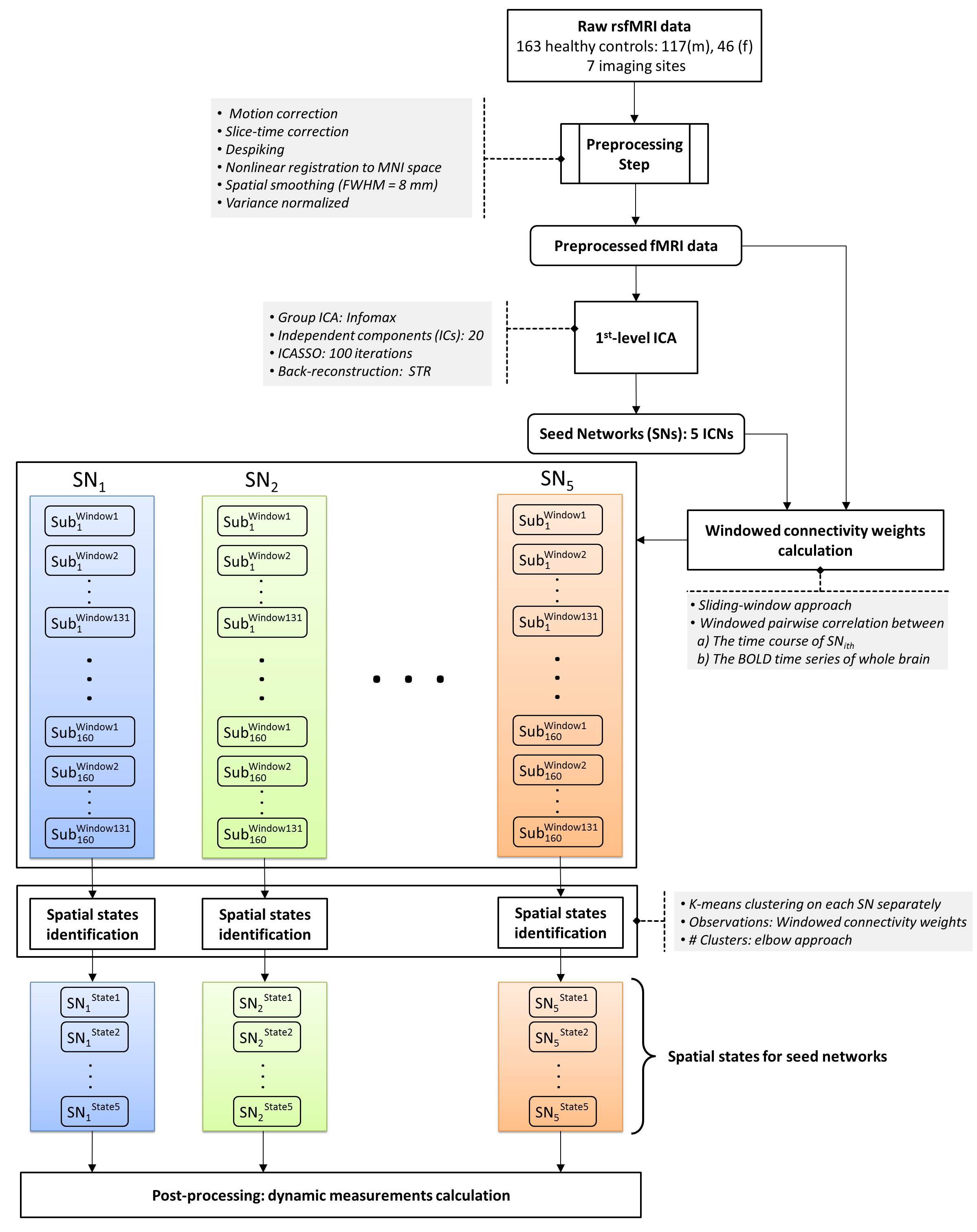
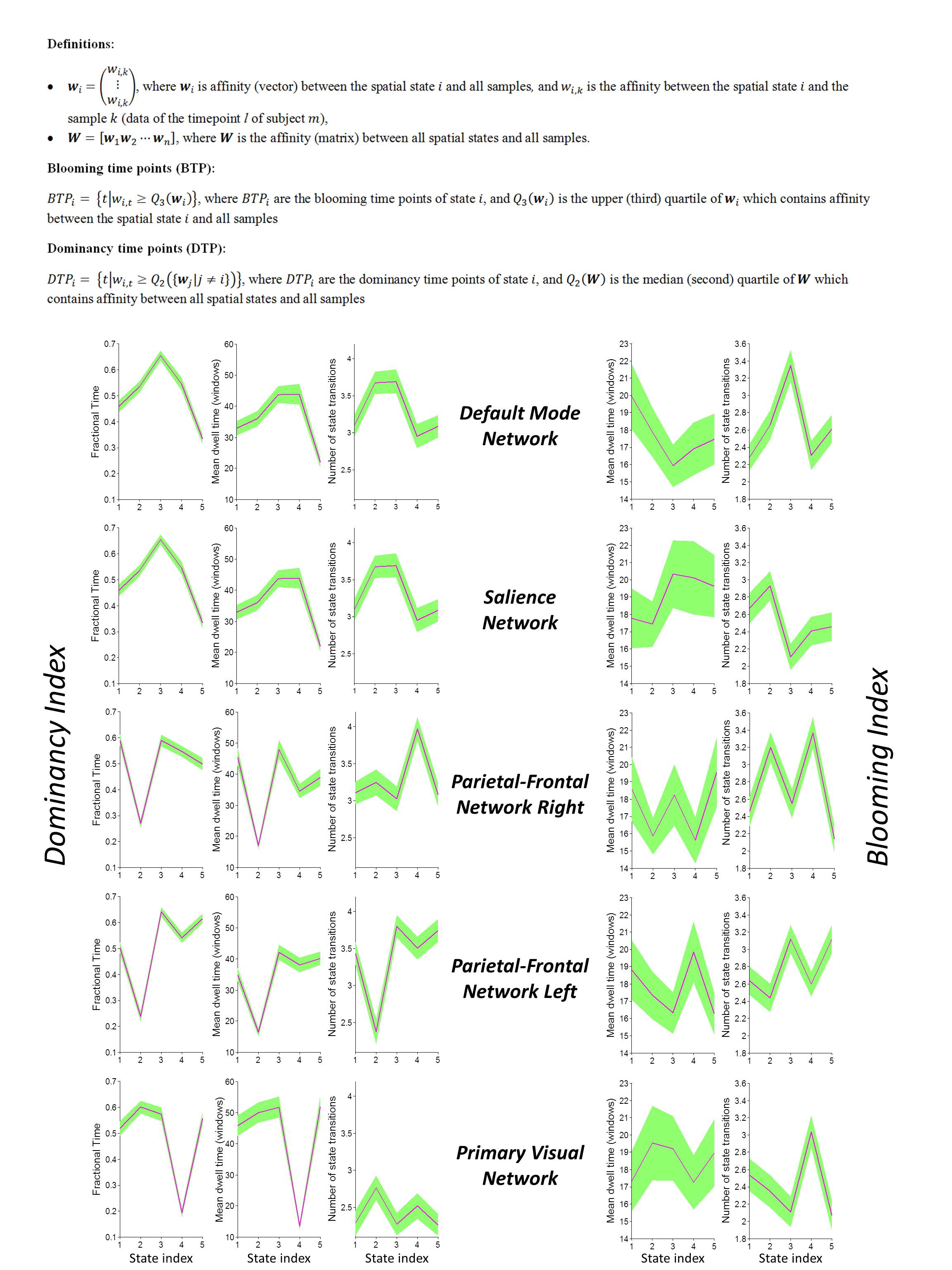
The dataset includes 163 healthy controls (female/male: 46/117) from 7 imaging sites. Data of each subject underwent a series of preprocessing steps (the analysis pipeline illustrated in Figure 1). The preprocessed data were decomposed using first-level spatial-ICA and five previously established intrinsic connectivity networks (ICNs) were retained for further analysis (referred to as functional seed networks or simply fSNs hereon). In contrast to a ROI-based approach, this ensures all the seed networks show similar functional behavior over time. Next, sliding time window correlation was applied between the timecourse of each fSN and the BOLD timeseries of whole brain voxels to obtain networks that show spatial variation over time (windowed-CWs). K-means clustering was implemented to identify the spatial states of each fSN. For each window, the similarity of windowed-CWs to each spatial state was computed (affinity matrices). The dynamic characteristics of the brain were evaluated using the spatial maps of the spatial states for spatial coupling and using the affinity matrices for temporal coupling. For post-processing, two complementary metrics, blooming and dominancy, were introduced to extract the temporal properties of the fSNs. Blooming timepoints of state i are the timepoints with a stronger association of state i with data compare to its associations at other timepoints. Dominancy timepoints are the timepoints in which state i is stronger than average of all other states of all time. The temporal dynamic information of spatial states was evaluated using both state-level and meta-state analysis.

Results

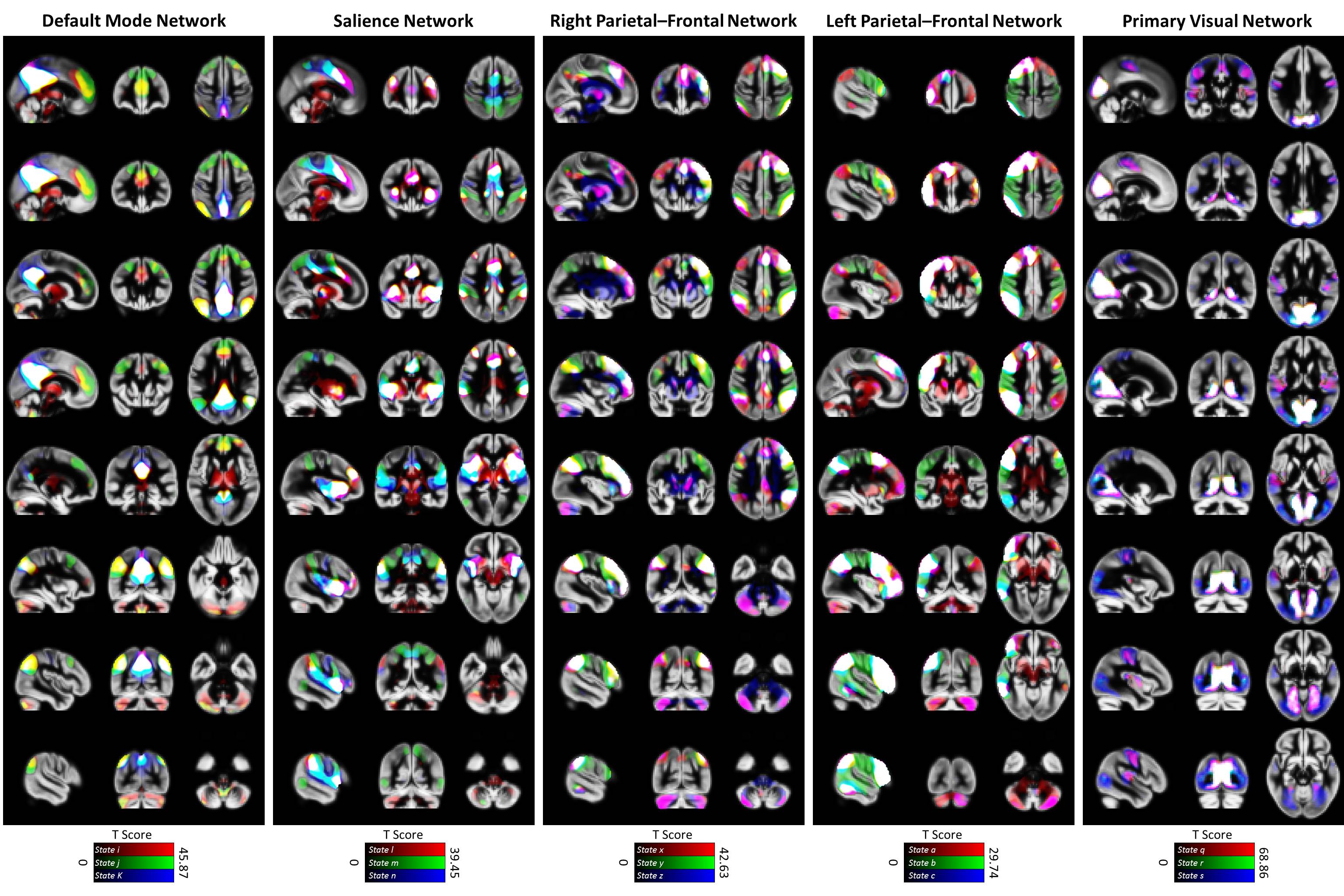
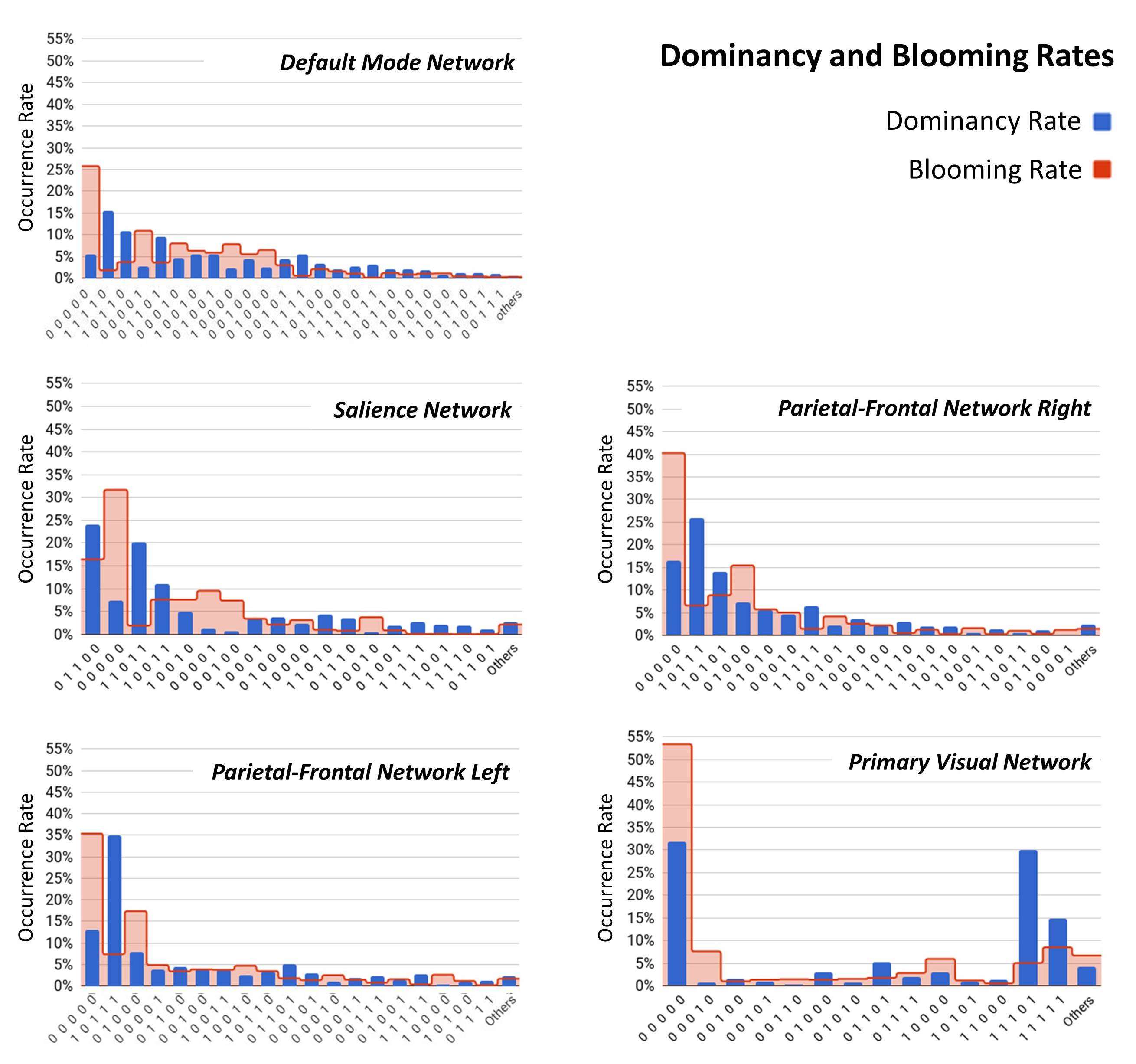
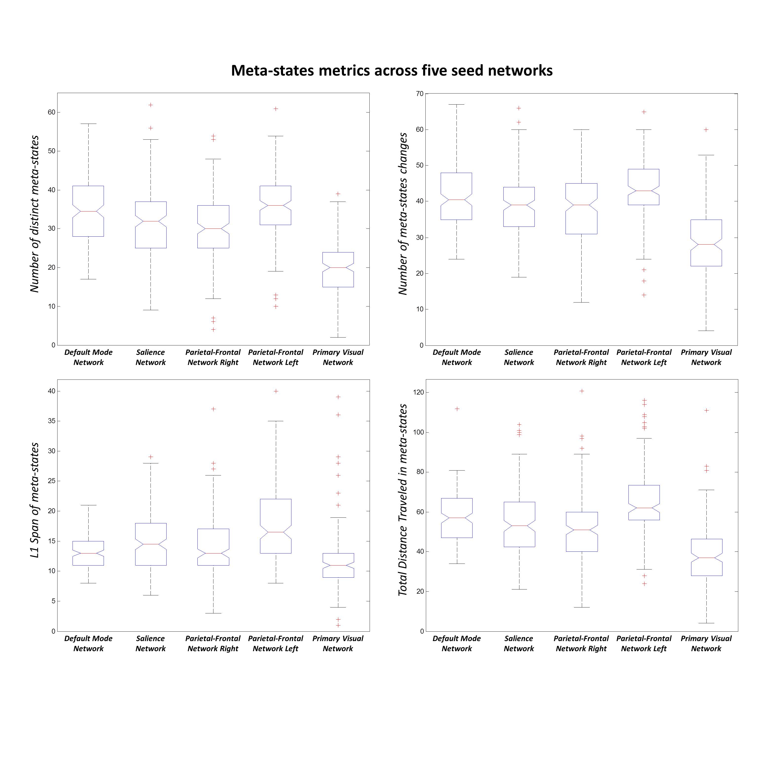
Three subjects were disregarded due to poor quality. Five major ICNs, including the DMN, salience network, right and left parietal-frontal networks, and primary visual network, were selected as fSNs and their timecourses were used for further analysis. For each fSN, 131×160 windowed-CWs were calculated (131 windowed-CWs per subject) and used as the input for the states identification step. The elbow method selected the same number of spatial states (5 clusters) for all fSNs. Three arbitrarily-selected spatial states for each fSN are shown in Figure 3 demonstrating variations in spatial coupling of each fSN. We next present some examples of the time-varying characteristics that can be captured via the temporal information of the spatial states (Figures 2, 4, and 5). One advantage of this work is providing the dynamic indices for fSNs (Figures 2 and 5). This provides a rich set of time-varying characteristics that include system-specific dynamic information. For instance, our analysis reveals that the spatial state #3 of the DMN has the highest dominancy rate with the maximum number of blooming transitions. This suggests that the spatial state #3 acts as the base for the DMN chronnectome (Figure 2). Interestingly, the spatial state #3 has the maximum spatial similarity (correlation value = 0.85) with the static DMN (other spatial states ranged between 0.61-0.76). Combining the information obtained from this approach with the global brain dynamic information obtained from others approaches can enhance our understanding of the chronnectome. In addition, although we evaluated the dynamic information of each fSN separately, the spatiotemporal information of fSNs can be combined and analyzed together to provide a richer understanding of the brain chronnectome.

Discussion and Conclusion

We introduced a novel framework for analyzing spatiotemporal dynamic of the brain. The findings reveal a set of distinct spatial patterns with unique temporal characteristics for each ICN. This emphasizes on the ability of our approach in capturing spatial and temporal variations of brain functional organizations. The initial results show the benefits of capturing the spatiotemporal variations of functional connectivity at macroscale and further improving our knowledge in this realm. Further investigations are needed to uncover the underlying causes and functional relevance. Next steps include evaluating the relationship between the information obtained using this approach and various demographics (age and gender) as well as pathophysiology characteristics.

Acknowledgements

No acknowledgement found.

References

1. Calhoun, V.D., et al., The chronnectome: time-varying connectivity networks as the next frontier in fMRI data discovery. Neuron, 2014. 84(2): p. 262-74.

2. Hutchison, R.M., et al., Dynamic functional connectivity: promise, issues, and interpretations. Neuroimage, 2013. 80: p. 360-78.

Figures

Figure 1. Schematic of the analysis pipeline. Preprocessing was performed on the resting-state functional magnetic resonance imaging (rsfMRI) data. Spatial independent component analysis (ICA) was performed to extract intrinsic brain networks (ICNs). Five major ICNs were selected as the seed networks (SNs) for further analysis. Using sliding-window approach and Pearson correlation, the whole brain connectivity weights of each SN were calculated at each time window. K-means clustering was applied on the connectivity weights of each SN to identify the spatial states of the SN. Post-processing was applied on the temporal information of spatial states to capture their temporal variations.

Figure 2. The approach allows studying the time-varying characteristics of the brain at system-specific and global levels using the temporal information of spatial states. Two complementary metrics, blooming and dominancy, were introduced to extract different time-varying information of seed networks. The red line is the mean value of each calculated index for each metric and the green area is mean ± standard deviation. The weight of state i at a BTP is larger than the 75% of all weights of that state. The weight of state i at DTP is larger the 50% of weights from all other states.

Figure 3. RGB color-code presentation of three arbitrarily-selected spatial states for five brain networks. Red, blue, and green represent the strength of three spatial states. Thus, for instance, white represents the areas in which the brain network is strong in all three spatial states, and yellow shows strong association in red and green spatial states. It worth mentioning that the spatial states of different SNs were identified independently; therefore, for example, the first spatial state of SN_i is not correspondent with the first spatial state of SN_j (i ≠ j).

Figure 4. An example of the time-varying findings that we can obtain from the temporal information of spatial states. Each bar presents the occurrence rate (incidence) of the dominancy (blue) and blooming (red) metrics for the corresponding states combination. For instance, the results show that the default mode network dominancy mode is more spread across various state combinations while the primary visual network has three significant combinations.

Figure 5. Meta-state level analysis of brain dynamic. Using the proposed approach, we can compare the meta-state measures across different seed networks and groups. For instance, our results show that the default mode network has a low variation across healthy subjects, and the primary visual network has lower dynamic variation among five selected seed networks while it has a high variability across subjects.

Proc. Intl. Soc. Mag. Reson. Med. 26 (2018)

1216