1213
MouseStream: A Software Suite for Mapping and Analyzing Mouse Cortical Functional Architecture In Vivo Using Magnetic Resonance Microscopy1Department of Biomedical Engineering, Columbia University, New York, NY, United States, 2Departments of Neurology, Columbia University College of Physicians and Surgeons, New York, NY, United States, 3Departments of Neurology, Radiology or Psychiatry, Columbia University College of Physicians and Surgeons, New York, NY, United States
Synopsis
The functional architecture of the cortex has never been mapped in vivo with the fidelity necessary to distinguish “functional unit”. Mapping the functional architecture of the cortex, reflecting the observed regional and layer differences in synaptic density and its correlate energy metabolism, has been very challenging. Here we set out to address this issue by in vivo high-resolution cerebral blood volume (CBV) mapping of the mouse cortex. Tailored software, MouseStream, was developed to reconstruct the cortical CBV data through the normalized curved cortical coordinate (NCCC). NCCC allows projection of functional architectures mapped using CBV onto the cortical surface across the whole cortex and from different cortical depths.
INTRODUCTION
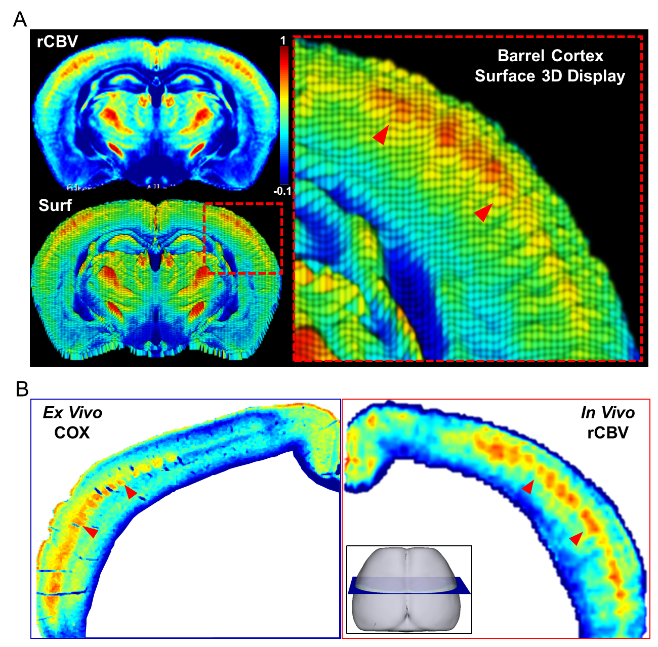
The functional architecture of the cortex reflects cellular compositions and metabolic states that vary across the cortical surface and among its different layers. The cortical functional architecture has never been mapped in vivo with the fidelity necessary to distinguish “functional unit”. Here we address this issue by in vivo high-resolution relative cerebral blood volume (rCBV) mapping1 and generated microscopic three-dimensional functional maps of the cortex in the living mouse.
Mapping the cortical functional architecture, reflecting regional and layer differences in synaptic density and its correlate energy metabolism, has been very challenging. Tailored software, MouseStream, was developed to address this challenge through the normalized-curved-cortical coordinate (NCCC).
METHODS
A Bruker BioSpec 9.4T system was used with a 23mm 1H circularly-polarized transmit/receive capable mouse head volume coil. Mice were anesthetized using the medical air and isoflurane. T2-weighted images were acquired before and 36-min after intraperitoneal injections of the contrast agent Gadodiamide at the dosage of 10 mmol/kg. T2-weighted images were acquired with RARE (TR/TE: 2,500/45 ms; RARE factor, 16; in-plane resolution, 50 µm; slice thickness, 250 µm), from 10 wildtype (C576BJ) mice in total.
As previously described1, rCBV was mapped according to changes in the transverse relaxation time (∆R2) induced by the contrast agent. rCBV images were preprocessed with skull stripping, large vessel filtering, isotropic up-sampling and co-registered into a common template space2.
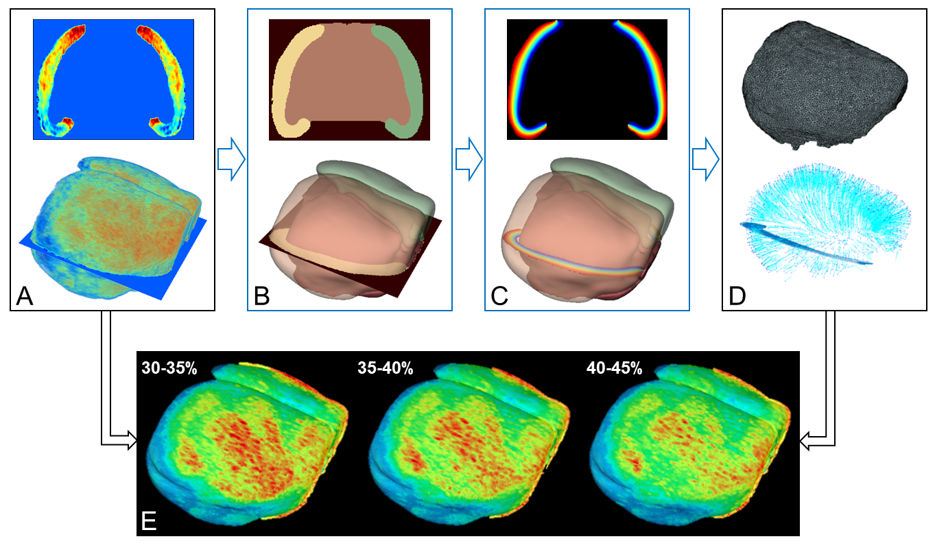
Co-registered rCBV volumes in Euclidean coordinate have to be first transformed to the NCCC, which aligns better with the cortical anatomy. The proposed pipeline is illustrated in Figure-2. We used a similar technique as mapping mouse cortical thickness by solving the Laplace’s equation3,4. This was the first time applying this technique in this context to process in vivo functional MRI data of the mouse brain.
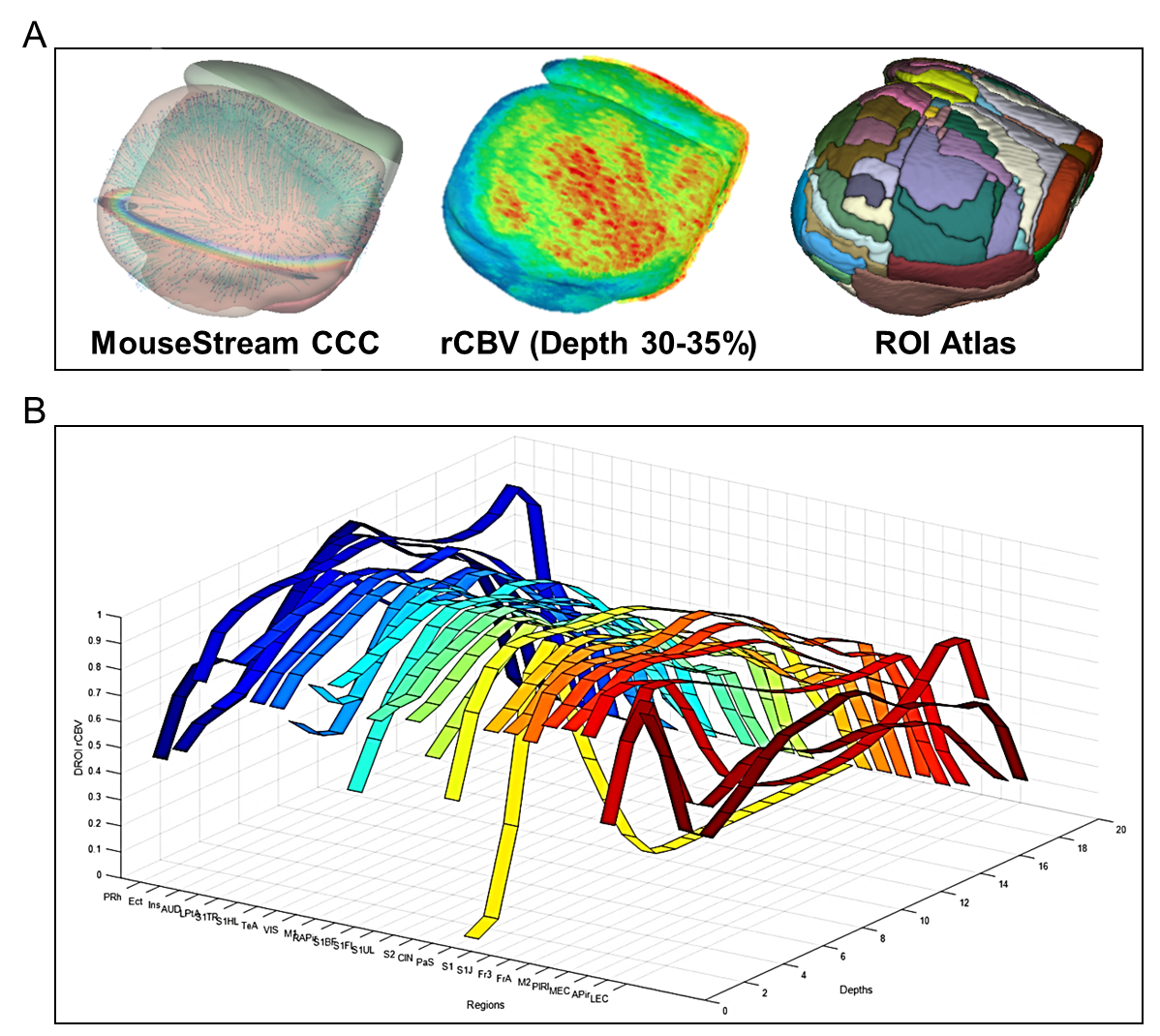
The cortical functional architecture patterns we observed vary by cortical depths and regions. A whole brain depth & region of interest (DROI) analysis was performed to illustrate those features. MouseStream also generates the cortical thickness map as one output.
To visualize the whole cortex in one view, flat maps can be generated for both cortical rCBV and the thickness.
RESULTS
Figure-1 shows a typical group-wise in vivo rCBV map compared with the ex vivo COX staining.
The proposed pipeline is illustrated in Figure-2.
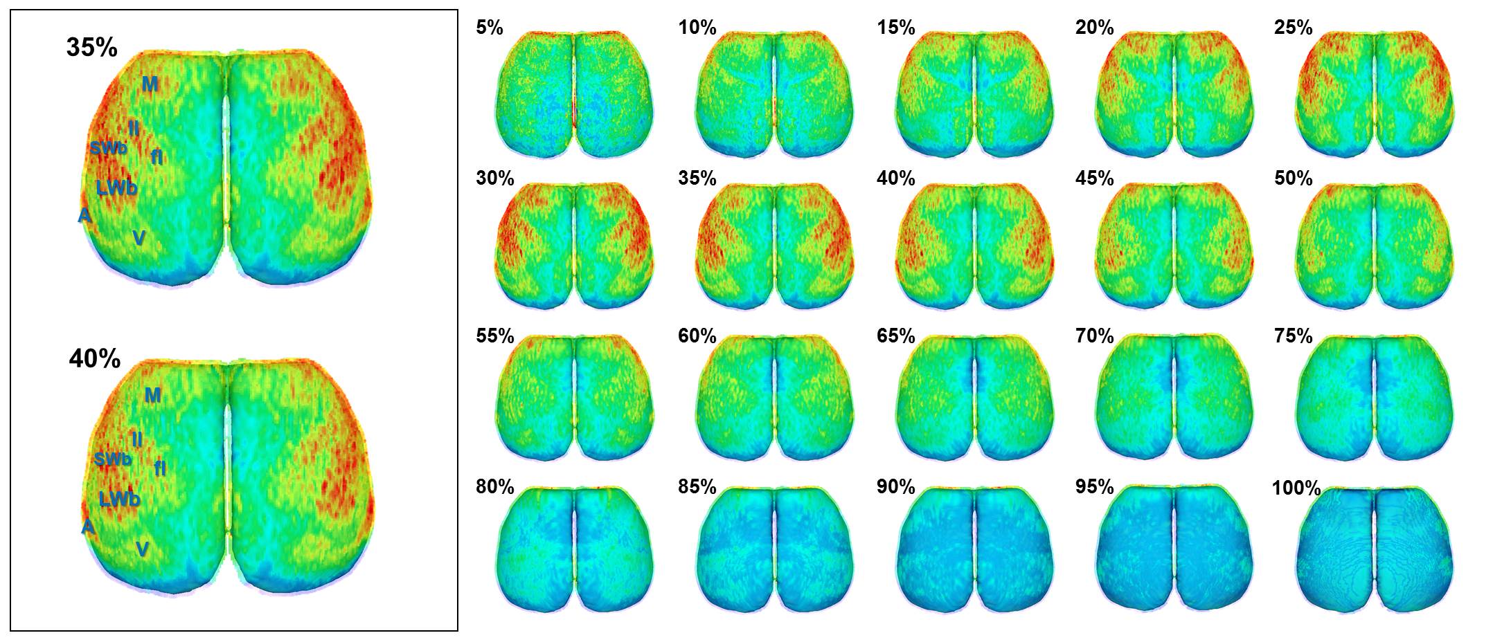
rCBV surface projection results generated by MouseStream at 20 depths of the cortex are displayed in Figure-3.
Figure-4 shows cortical DROI results of rCBV calculated from 20 depths and 26 regions.
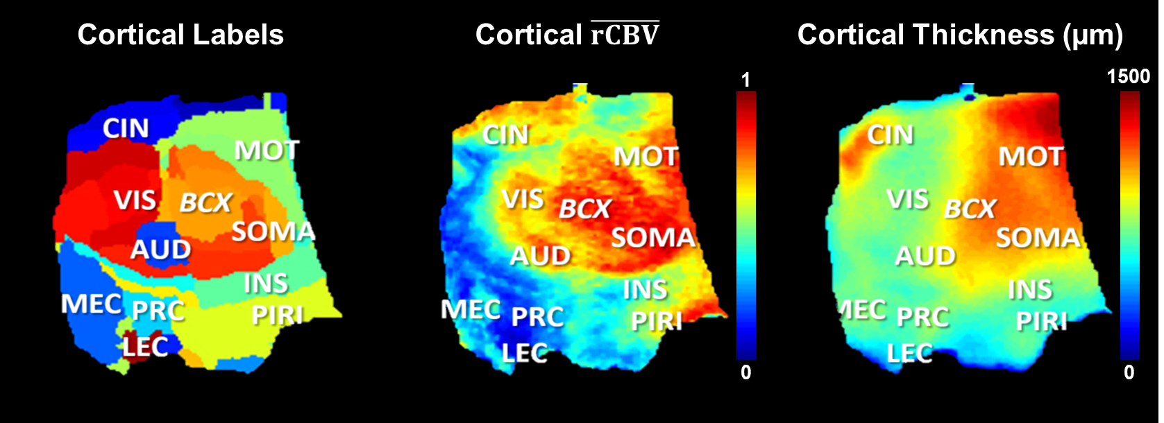
Figure-5 shows the flap maps of cortical labels, rCBV and thickness.
DISCUSSION
MouseStream utilizes the high contrast, high-resolution rCBV maps in vivo and is capable to map the three-dimensional functional architecture of the whole cortex noninvasively, across the cortical surface and among its different depths.
Besides providing insight into the cortical organization, MouseStream allows a more precise spatial-temporal mapping of how the brain changes its function and structure in response to experience. And more importantly, being able to map function and structure simultaneously opens up the opportunity to better understand the functional-structural relationships in neuroplasticity.
CONCLUSION
We have successfully mapped the in vivo functional architecture of the mouse cortex across its surface and among its different depths for the first time, using rCBV as the image contrast. MouseStream provided an automated processing, analysis and visualization pipeline for mapping mouse cortical functional architecture in vivo. Surface-based vertex-wise data comparisons can be easily applied.
Besides clarifying the functional organization of the cortex, we believe that the more important application of the reported MRI tools is to map functional changes over time. When investigating brain function and how and where it changes with experience, the MRI tools add an important complement to electrophysiology and confocal microscopy.
Acknowledgements
No acknowledgement found.References
1. Moreno, H., Hua, F., Brown, T. & Small, S. Longitudinal mapping of mouse cerebral blood volume with MRI. NMR Biomed 19, 535-543 (2006).
2. Avants, B.B., et al. A reproducible evaluation of ANTs similarity metric performance in brain image registration. Neuroimage 54, 2033-2044 (2011).
3. Jones, S.E., Buchbinder, B.R. & Aharon, I. Three-dimensional mapping of cortical thickness using Laplace's Equation. Human Brain Mapping 11, 12-32 (2000).
4. Lerch, J.P., et al. Cortical thickness measured from MRI in the YAC128 mouse model of Huntington's disease. Neuroimage 41, 243-251 (2008).
Figures