1143
Quantitative Modeling of Glymphatic Pathways of the Brain Using MRI1Neurology, henry ford health system, detroit, MI, United States, 2Neurology, Wayne State University, detroit, MI, United States, 3Physics, Oakland University, Rochester, MI, United States
Synopsis
The dynamic exchange of CSF with ISF is identified as the glymphatic system. The impairment of the glymphatic clearance is involved in the development of neurodegenerative conditions. Despite many recent studies that investigated the glymphatic system, few studies have tried to use a mathematical model to describe this system, quantitatively. In this study, we aim to model the glymphatic system from the kinetics of GD-DTPA tracer in order to 1) map the glymphatic system pathways, 2) derive kinetic parameters of the glymphatic system, and 3) provide quantitative maps of the structure and function of this system.
INTRODUCTION
Recent studies1 have reformed the traditional model of cerebrospinal fluid (CSF) hydrodynamics. The dynamic exchange of CSF with ISF is identified as the glymphatic system. The impairment of the glymphatic clearance is involved in the development of neurodegenerative conditions, including diabetes, Alzheimer`s disease, traumatic brain injury (TBI), stroke and glaucoma1,2. Now, it has been revealed that the glymphatic system circulates through the para-vascular (para-arteries and para-veins) pathways3-5, supported by two-photon imaging of live mice brain4. Despite many recent studies that investigated the glymphatic system, few studies have tried to use a mathematical model to describe this system, quantitatively6. In this study, we aim to model the glymphatic system using the kinetics of GD-DTPA tracer in order to 1) map the glymphatic system pathways, 2) derive kinetic parameters of the glymphatic system, and 3) provide quantitative maps of the structure and function of this system. We use the MRI data of healthy and Diabetes mellitus (DM) animals to assess the performance of the model in differentiating affected tissues.METHODS
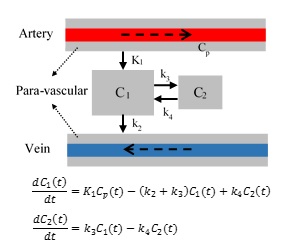
Image acquisition. 8 rats (4 controls and 4 diabetics) followed in a CE-MRI protocol using Gd-DTPA contrast agent (CA)2. T1-weighted images were acquired using a 7Tesla animal scanner with TR/TE=15/4ms and acquisition voxel size of 0.125×0.167×0.167 mm3 and reconstructed to 0.125×0.125×0.167 mm3. Up to 62 time volumes were acquired until 6 hours after intra-cisterna magna (ICM) contrast agent delivery. This enabled us to monitor the propagation profile of the tracer in the brain during the experiments. For each voxel, x, the intensity value at each time, Ix(t), is used to derive time signal curve (TSC)6 representing the time profile of the tracer’s density, TSCx(t)=100(Ix(t)- Ix(t0))/Ix(t0). Pre-Processing. For each case, the non-brain tissues were masked. Then, all the volumes of each case were co-registered to the first time point using rigid transformation computed in SPM8. Next, we clustered the voxels of each brain into similar regions based on the propagation profile of the tracer during the experiment using k-means clustering in MATLAB. This reduced the computations as well as reducing the effect of noise and uncorrected head motions. Proposed model. As suggested by 6 we used a 2-tissue multi-compartment model shown in Fig. 1. Using Laplace transform, the solution for the differential equations is C(t)=C1(t)+C2(t)=0.5K1[(1+A).exp(-(B+M)t)+(1-A).exp(-(B-M)t)]*Cp(t) in which * represents mathematical convolution, 4M2=(k2+k3+k4 )2-4k2 k4, A=0.5×(k2-k3-k4)/M, and B=(k2+k3+k4)/2. Benefiting from clustering the tissues based on the dynamic response of the tissues to the CA infusion, we defined an approach to find the input function for each region. First, for each region (cluster), the neighboring regions were found based on their shared boundaries. Then, among those neighboring clusters, the cluster that dominantly drives that region was found based on 1) the arrival time, ta, of CA to each region, 2) the rising slope of TSC after injection, and 3) the time that the TSC reach to its maximum. Finally, employing a non-linear least square optimization tool in MATLAB, we estimated the unknown parameters for each cluster. Two quantities 6 were calculated from the estimated parameters: retention=k3/k4 and loss=k2/(1+k3/k4) 6. ‘Retention’ is assumed to characterize the fraction of the tracers that remain bonded with large molecules and thus can reduce the CSF speed. ‘Loss’ measures the portion of particles that continue to flow through the glymphatic system by going back to the para-veins.RESULTS
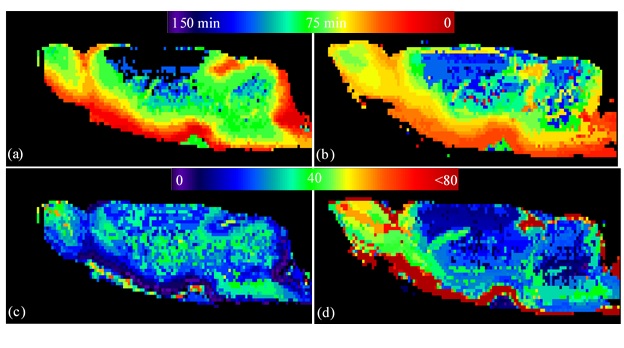
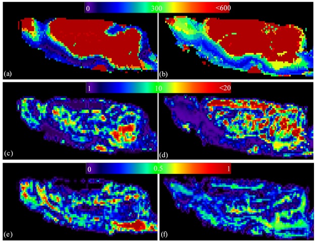
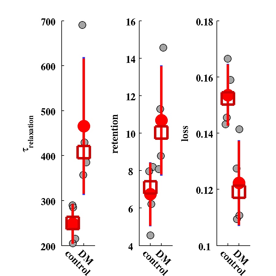
The maps of two experimental parameters i.e., the CA arrival time (ta) and the CA residual maps for two typical cases (one healthy control and one DM animal) are shown in Fig. 2. It can be seen that the tracer takes longer to reach to the anterior-frontal paravascular spaces in the DM animal; suggesting lower bulk speed of CSF in the para-vasculatures. Moreover, much higher amount of the tracer has remained in the DM brain at the end of experiment. In Fig. 3 the estimated parameters of the 2-tissue kinetic model as well as a simple one-exponential model are shown. The corresponding quantitative values of these three parameters for all the animals are plotted in Fig. 4. It can be seen that in the DM animals the clearance time constant and the retention were increased and the loss was decreased compared with healthy control animals, significantly.DISCUSSION and CONCLUSION
These evidences are consistent with previous findings that suggest the waste clearance gets slower in diabetes. Modeling glymphatic system using dynamics of the tracer can reveal characteristic maps of the paravasculatures. The resulted parameters may be used in diagnosis and treatment evaluation of brain diseases.Acknowledgements
This work was supported in part by NIH grants, RF1 AG057494, RO1 NS097747 and R21 AG052735.References
1. Iliff JJ, Wang M, Liao Y, et al. A paravascular pathway facilitates CSF flow through the brain parenchyma and the clearance of interstitial solutes, including amyloid beta. Science translational medicine. 2012;4(147):147ra11.
2. Jiang Q, Zhang L, Ding G, Davoodi-Bojd E, Li Q, Li L, et al. Impairment of the glymphatic system after diabetes. J Cereb Blood Flow Metab. 2017;37(4):1326-37.
3. Kiviniemi V, Wang X, Korhonen V, Keinanen T, Tuovinen T, Autio J, et al. Ultra-fast magnetic resonance encephalography of physiological brain activity - Glymphatic pulsation mechanisms? J Cereb Blood Flow Metab. 2016;36(6):1033-45.
4. Nedergaard M. Neuroscience. Garbage truck of the brain. Science. 2013;340(6140):1529-30.
5. Taoka T, Masutani Y, Kawai H, Nakane T, Matsuoka K, Yasuno F, et al. Evaluation of glymphatic system activity with the diffusion MR technique: diffusion tensor image analysis along the perivascular space (DTI-ALPS) in Alzheimer's disease cases. Japanese journal of radiology. 2017;35(4):172-8.
6. Lee H, Xie L, Yu M, Kang H, Feng T, Deane R, et al. The Effect of Body Posture on Brain Glymphatic Transport. The Journal of neuroscience : the official journal of the Society for Neuroscience. 2015;35(31):11034-44.
Figures