Synopsis

Conventional MR images and pseudo-CT’s (pCT’s) generated using state-of-the-art machine learning techniques poorly characterize bone anatomies, preventing applicability for orthopedic applications. We hypothesize that smart use of several specific MR contrasts will expose the information needed for diagnostic quality bone visualization. We designed a patch-based convolutional neural network taking groups of different MR contrasts -which were obtained from a single multi-gradient sequence- as inputs . It generated competitive pCT scans, capturing local anatomical variances present in the dataset. We show that Dixon reconstructed inputs appear to generate better soft-tissue visualization, while complex-valued data show promising results in bone reconstruction.

Introduction

Methods aiming at obtaining electron density information from MRI have gained a lot of attention in the last decade, particularly for PET-MRI attenuation correction¹ and MRI-only radiotherapy treatment planning (RTP)². More recently, MRI-based visualization and characterization of the osseous structures³ and surrounding soft tissues are being investigated. This could improve diagnosis and treatment guidance for orthopedic purposes. For instance, femoral acetabular impingement is a condition affecting the hip joint, in which combined visualization of osseous and soft tissues is needed for an accurate choice of treatment. Currently, a trend can be observed towards the use of deep learning for pseudo-CT (pCT) generation, often using a single gradient echo image as input. We hypothesize that smart use of available MR data, such as complex data or Dixon reconstructions, could improve pCT quality. Although current deep learning techniques have demonstrated to fulfill the criteria needed for PET-MRI⁴ and RTP^5-6, they do not provide diagnostic quality bone visualizations or accurate 3D models of the osseous structures, which is required for orthopedic applications.

In this study, we investigate the influence of using different MR contrasts obtained from a single MRI sequence as input for a multi-channel convolutional neural network (CNN) on pCT prediction, focusing on bone reconstruction.

Methods

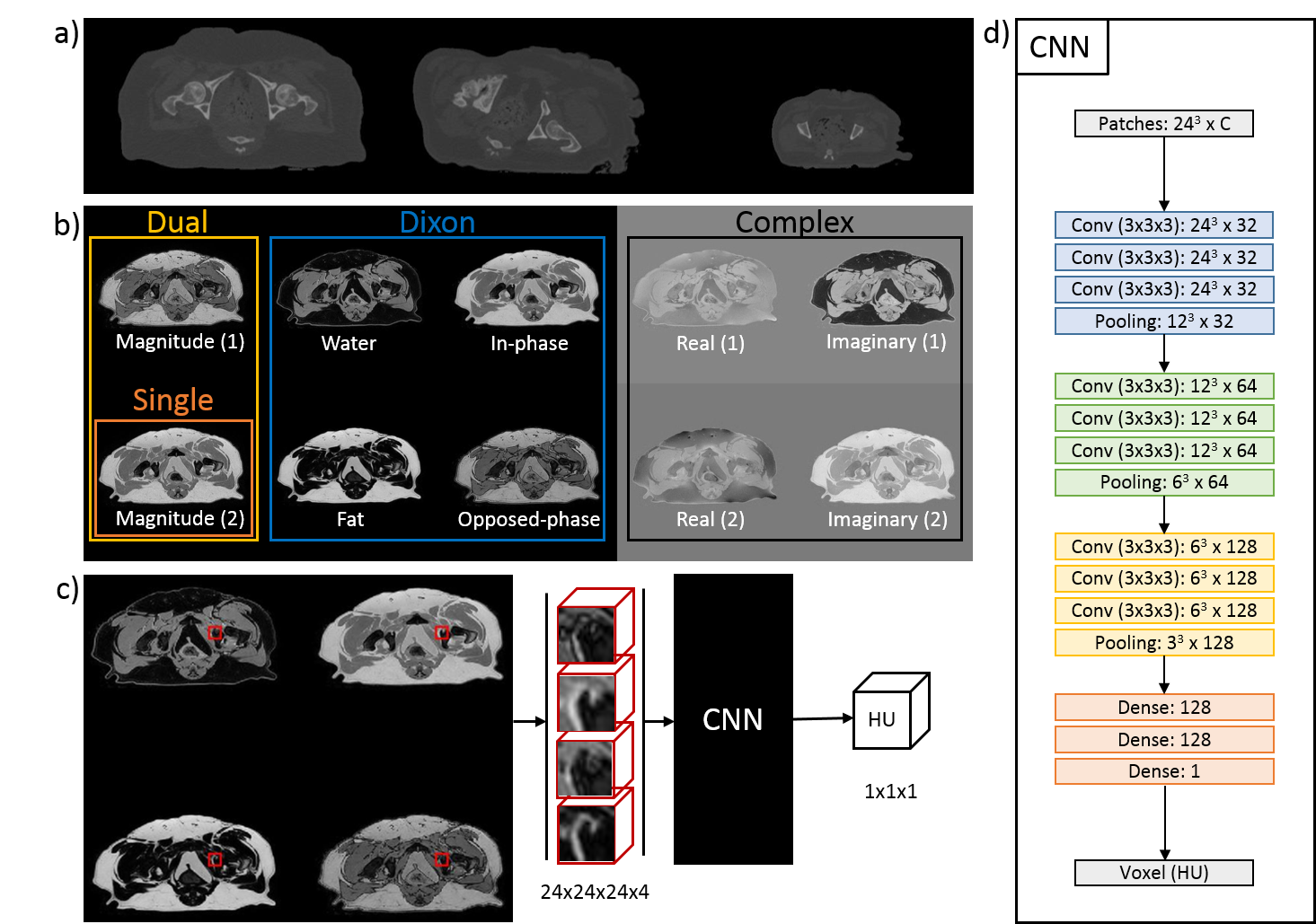
An ex vivo study was performed on 17 domestic dogs admitted to the veterinary department for scientific purposes, deceased of natural causes. Both CT (Brilliance CT big bore, Philips) and MRI (1.5T, Ingenia, Philips Healthcare, Best, Netherlands) of the pelvic region were acquired in fixed supine positions. A variety of MR contrasts was generated using a 3D T1w dual gradient-echo with Dixon water-fat reconstruction. Imaging parameters included: TR/TE1/TE2 = 6.7/2.03/4.28ms; BW = 540 Hz/pix, acquired/reconstructed voxel: 1x1x1.34mm / 0.6x0.6x0.67mm; FOV = 270x270x120mm. CT slice spacing was 0.7 mm and pixel spacing ranged between 0.4/0.8 mm. CT data was registered non-rigidly to MRI to create voxelwise matching MRI-CT data for training.

For pCT generation, we used the patch-based CNN presented in Figure 1d which was trained to learn a mapping from MR contrasts to CT Hounsfield units (HU). Because of the anatomical variations in the dataset (Figure 1a), the patch size was limited to 24x24x24 voxels to increase sensitivity to local structures instead of large anatomies (Figure 1c). To study the effect of MR contrasts on pCT generation, the CNN has been trained with four combinations of images reconstructed from the dual echo MRI scan: one single magnitude image from echo 2 (Single echo), magnitude images from both echoes (Dual echo), complex-valued data (Complex), and Dixon reconstructions (Figure 1b). The resulting pCTs were quantitatively evaluated against the real CT image using mean absolute error (MAE) and Dice coefficient on bone segmentations and qualitatively by manual inspection of the pCTs. A three-fold cross validation assessed the predictive power of the networks.

Results

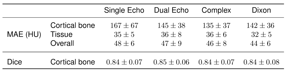
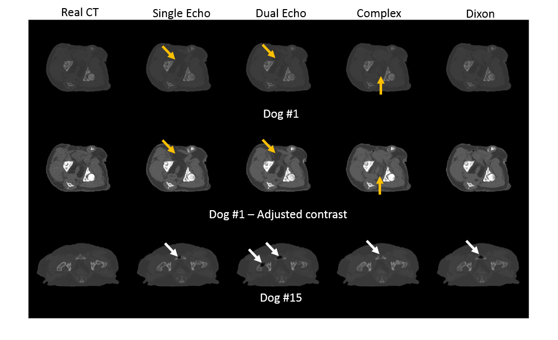
For each input combination, we show the quantitative (Figure 2) and qualitative (Figure 3) results. These results demonstrate that our network is competitive with other deep learning techniques². Both figures also indicate differences in prediction quality, with a better prediction of HU in soft tissue when using Dixon inputs (MAE_tissue and yellow arrows), and in cortical bone when using complex-valued inputs (MAE_bone and white arrows).

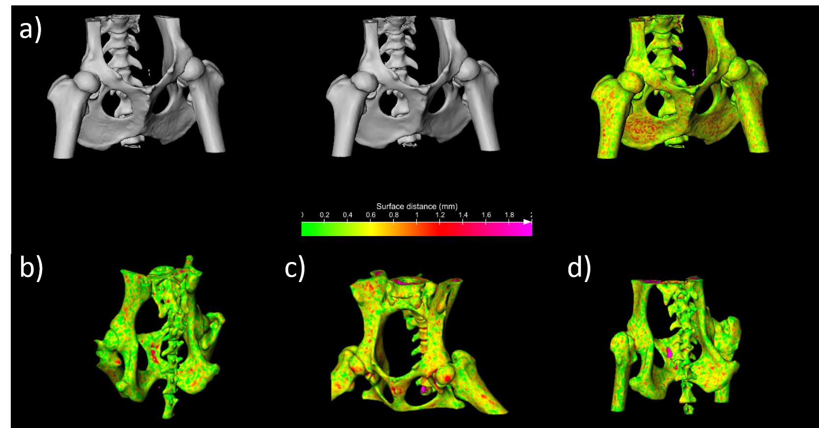
In an orthopedic perspective, Figure 4 and 5 show a comparison between the CT and pCT obtained on dog #13. High resemblance is demonstrated by the gif in Figure 4. The color-coded point-to-point distance map in Figure 5 demonstrates sub-millimeter accuracy compared to the registered CT, which is very promising for the detection of bone abnormalities and for 3D modeling of patient-specific instruments.

Discussion

Although trained with small receptive fields, the network we designed is competitive with other deep learning techniques and captures anatomical details within subjects with large variations in size. Particularly for orthopedic purposes this is promising, as pathologies often manifest as small changes in osseous structures.

The type of input data and the number of channels of the CNN were shown to influence the outcome of the pCT predictions. These results strongly suggest that the entire workflow, from data acquisition to network architecture, can be tuned to obtain optimal results for a specific application. For orthopedic purposes, complex-valued MR contrasts provided encouraging results in characterizing cortical bone and facilitating 3D renderings of the osseous structures.

Further studies should investigate the relation between the nature and amount of the MR inputs and the architecture of the network. Nonetheless, the method we designed was demonstrated to generate state-of-the-art bone visualization, paving the way for MRI-based treatment guidance for orthopedic purposes.

Acknowledgements

References

1. Keereman V, Fierens Y, Broux T, De Deene Y, Lonneux M, Vandenberghe S. MRI-Based Attenuation Correction for PET/MRI Using Ultrashort Echo Time Sequences. J Nucl Med. 2010;51(5):812–8.
2. Edmund JM, Nyholm T. A review of substitute CT generation for MRI-only radiation therapy. Radiat Oncol. 2017;12(1):28.
3. Tadros A, West, J, Nazaran A, Ma YJ, Hoenecke H, Du J, Chang E. 3D IR-UTE-Cones for high contrast MR imaging of lamellar bone. In proceedings of the 25th Annual Meeting of ISMRM, Honolulu, Hawai, 2017:5019
4. Liu F, Jang H, Kijowski R, Bradshaw T, McMillan AB. Deep learning MR imaging-based attenuation correction for PET/MR imaging. Radiology. 2017, Ahead of print.
5. Han X. MR-based synthetic CT generation using a deep convolutional neural network method. Med Phys. 2017;44(4):1408–19.
6. Nie D, Xiaohuan C, Gao Y, Wang L, Shen D. Estimating CT Image from MRI Data Using 3D Fully Convolutional Networks. MICCAI 2016 DL Workshop, Athens, Greece, 2016;10008:197–205.