1034

Prostate microstructure specificity with diffusion relaxometry

Gregory Lemberskiy^1,2, Els Fieremans¹, Jelle Veraart¹, Andrew B. Rosenkrantz¹, and Dmitry S Novikov¹

¹Radiology, NYU School of Medicine, New York, NY, United States, ²Sackler Institute of Graduate Biomedical Sciences, NYU School of Medicine, New York, NY, United States

Synopsis

We identify the contributions of prostate cellular and glandular compartments to the overall diffusion time-dependent diffusion tensor, by varying echo time and relying on their different T2 values. We test the functional form of compartment tensor eigenvalues with respect to the diffusion time against a variety of tissue models, and find the glandular tissue being best described by the short-time surface-to-volume limit, whereas the random permeable barrier model is most applicable in cellular tissue, and for tumors of various grade. Our framework allows quantification of glandular sizes, cellular fiber diameters, membrane permeability, compartment T2-values, and volume fractions.

Introduction

The apparent diffusion coefficient (ADC) is a highly sensitive biomarker for identifying prostate cancer¹. Though much of the literature reports ADC² as a measurement of cellularity, a side-by-side comparison³ of cellularity and volumetric changes in epithelium, stroma, and gland compartments revealed that the volume fractions alone explain most of the ADC contrast. Moreover, changes in compartment volume fraction correlate significantly with prostate cancer progression³. Though ADC is sensitive, it is not specific to the relative compartment contributions of the microstructural changes. In this study, we utilize the large differences⁴ in T2 to isolate tissue compartments in order to study their diffusion properties separately. We model multi-compartment signal:$$S(b,t,T_\text{E})=S_0\sum_c\,f_c\,e^{-T_\text{E}/T_2^c-bD_c(t)+\mathcal{O}(b^2)}\tag{1}$$in 3 dimensions of parameter space: diffusion time $$$t$$$, diffusion-weighting $$$b$$$, and echo-time $$$T_\text{E}$$$, that allows us to study compartmental diffusion and derive physical properties of each tissue compartment’s microstructure.

Methods

MRI: A multi-parametric diffusion STEAM acquisition, with $$$b=500\,\text{s/mm}^2$$$ along$$$\,17\,$$$directions and$$$\,2\text{ nominal}\,b=0$$$ images, which actually ranged from $$$[b=3-102\,\text{s/mm}^2],\,8\,$$$diffusion times:$$$\,t=[25.2-740\text{ms}]\,$$$using 8 mixing times$$$\,T_{\text{M}}\,=\,[6.38-719.32]\,\text{ms}$$$, and $$$3\,T_\text{E}=[52,115,180]\,\text{ms}$$$, was used to image$$$\,3\,$$$volunteers, on a Siemens 3T PRISMA system.

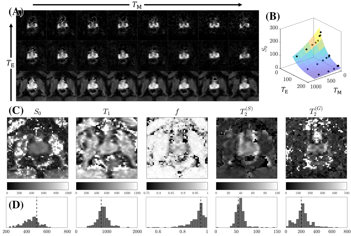
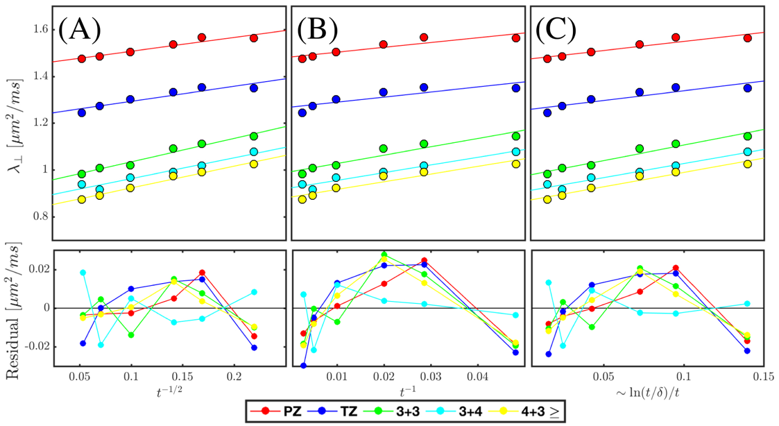
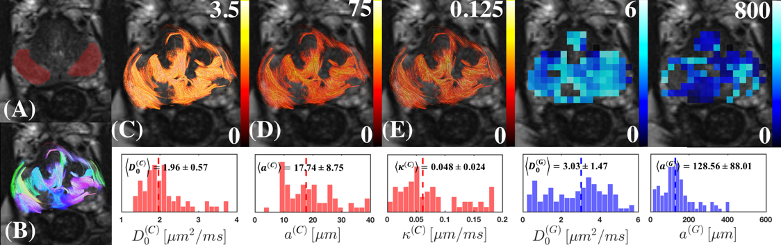
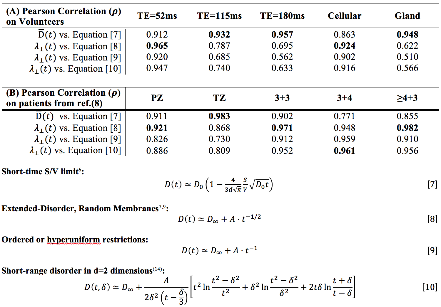
Modeling: The diffusion tensor from each acquisition is calculated to determine un-weighted$$$\,S|_{b=0}(T_\text{M},T_{\text{E}})$$$, which is modeled (Fig.2) using a$$$\,5\,$$$parameter model consisting of proton density$$$\,S_0$$$, cellular compartment fraction,$$$\,f$$$, cellular (fast) and glandular (slow)$$$\,T_2$$$, and single compartment$$$\,T_1$$$: $$S|_{b=0}=S_{0}e^{-T_\text{M}/T_1}\bigg(\underbrace{fe^{-T_\text{E}/T_2^{(C)}}}_{\textbf{C}}+\underbrace{(1-f)e^{-T_\text{E}/T_2^{(G)}}}_{\textbf{G}}\bigg)\tag{2}$$ These parameters were then recombined to estimate $$$T_\text{E}$$$-specific weights,$$W^{(C)}(T_\text{E})=\frac{C}{C+G},\quad\,W^{(G)}=1-W^{(C)}\tag{3}$$ which were subsequently used to extract diffusion tensors$$$\,D^{(C)}(t)\,$$$and$$$\,D^{(G)}(t)\,$$$corresponding to the cellular and glandular compartment from the overall diffusion tensor$$D(t,T_{\text{E}})=W^{(C)}(T_{\text{E}})\cdot\,D^{(C)}(t)+W^{(G)}(T_\text{E})\cdot\,D^{(G)}(t)\tag{4}$$$$\binom{D^{(C)}(t)}{D^{(G)}(t)}=\text{pinv}\left(\begin{bmatrix}W^{(C)}(T_{\text{E}_1})\,&\,W^{(G)}(T_{\text{E}_1})\\W^{(C)}(T_{\text{E}_2})\,&\,W^{(G)}(T_{\text{E}_2})\\\vdots&\vdots\\\,W^{(C)}(T_{\text{E}_\text{N}})\,&\,W^{(G)}(T_{\text{E}_\text{N}})\,\\\end{bmatrix}\right)\begin{bmatrix}\,D(t,T_{\text{E}_1})\\\,D(t,T_{\text{E}_2})\\\vdots\\\,D(t,T_{\text{E}_\text{N}})\,\\\end{bmatrix}\tag{5}$$ Where$$$\,t\sim\,T_\text{E}/2+T_\text{M}\,$$$and N=3 for our experiment. Eqn.5 separates the dependence of $$$T_\text{E}$$$ and$$$\,t\,$$$from$$$\,D\,$$$allowing for the evaluation of microstructural properties arising from those parameters. Probabilistic fiber tracking⁵, via MRTRIX3 (mrtrix.org), was performed on a dyadic tensor⁶ across 8 diffusion times on the cellular compartment.Compartmental tensors were then diagonalized for each $$$t$$$ to generate a set of eigenvectors and eigenvalues. The time-dependence of the eigenvalues from cellular, glandular, and overall-diffusion tensors at individual $$$T_\text{E}$$$ is evaluated [Table.1] using the short-time limit⁷, which depends on the free diffusivity,$$$\,D_0$$$, and surface-to-volume ratio, $$$S/V$$$, as well as with the long time limit, which depends on the finite bulk diffusion constant, $$$D_\infty$$$, the slope of the power law tail, $$$A$$$, and the power law scaling associated with the disorder geometry⁸, $$$\vartheta$$$:$$D(t)\simeq\,D_\infty+At^{-\vartheta}\tag{6}$$ For all assessments of the long-time limit,$$$\,\vartheta$$$, is fixed to study well established disorder geometries: extended disorder [Table.1,Eqn.[8]], hyper-uniform disorder [Table.1,Eqn.[9]], and short range disorder in 2-dimensions [Table.1,Eqn.[10]]. Additionally, the patient data (at low $$$T_\text{E}$$$) from ref.(7), which featured a diffusion STEAM acquisition at multiple $$$t$$$, is used to assess the power-law scaling in prostate tumors.

Results

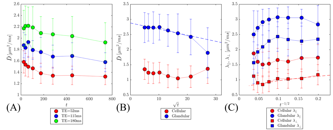
The functional form of $$$D(t)$$$ at various$$$\,T_\text{E}\,$$$changes [Figure.1(A)] from being well described by the long-time limit (stroma) at$$$\,T_\text{E}=52\,\text{ms}$$$ [$$$\rho=0.91$$$], to being poorly described by those same models at$$$\,T_\text{E}=180\,\text{ms}$$$ [$$$\rho=0.63$$$]. Conversely, correlation with the short time limit improves with longer $$$T_\text{E}=[52,115,180]$$$ resulting in $$$\rho=[0.91,0.93,0.96]$$$. Moreover, the value of the diffusion coefficient increases by as much as 59% between $$$\,T_\text{E}=52$$$ and $$$\,T_\text{E}=180$$$ ms. There is a factor of $$$\sim\,4$$$ difference in $$$T_2$$$ from cellular and glandular compartments [Fig.2] that facilitated the separation of diffusion compartments.

The cellular compartment and the patient tumor data is well described by extended disorder [Fig.3], prompting the use of the random permeable barrier model (RPBM)^10,11 to derive cellular diameters and cellular permeability [Fig.1(C), Fig.4)]. On the other hand, the poor fit of the gland compartment with long-time limits ($$$\rho=0.56$$$) and much better agreement with short time limit: $$$\rho=0.95$$$, prompted the use of the latter to derive glandular diameters [Fig.1(B), Fig.4].

The extracted stromal $$$(17.7 ± 8.8)$$$ and glandular diameters $$$(128.6 ± 88.0)$$$ were in good agreement with those reported in histopathology¹². Moreover, the cell membrane permeability $$$(0.048 ± 0.02)$$$ is similar to permeability measured from the red blood cell membrane¹³.

Discussion

This study emphasizes the importance of compartment $$$T_2$$$ weighing and the functional form of diffusion time dependence when modeling diffusion in prostate. Diffusion time-dependence is apparent at all $$$T_\text{E}$$$; however, there is a steady change in the functional form of $$$D(t)$$$ that reflects a different mixture of perceived microstructure [Table.1]. Diffusion through cellular tissue was best described with extended disorder, for which modeling permeability becomes necessary. This contradicts existing modeling philosophies,^15,16 which ascribe all diffusion time-dependence to a fully-restricted compartment. Changes in individual compartment volume fractions correlate strongly with cancer grade³. Our approach allow us to use diffusion to interpret changes from individual compartments, which could be useful in the clinic to study the progression of prostate cancer.

Conclusion

We presented a new method to (1) separate glandular and cellular compartments by exploiting their intrinsically different $$$T_2$$$ values; (2) determine their most appropriate microstructural models; and (3) to derive their relevant biophysical parameters, e.g., volume fraction, glandular size, cellular diameter, and membrane permeability.

Acknowledgements

We would like to thank Thorsten Feiweier for the development and support of the Siemens advanced diffusion WIP sequence.

References

1. Radiology ACo. MR Prostate Imaging Reporting and Data System version 2.0. Available at: http://www.acr.org/Quality-Safety/Resources/ PIRADS/. Accessed December 2015.

2. Chen L, Liu M, Bao J, et al. The correlation between apparent diffusion coefficient and tumor cellularity in patients: a meta-analysis. PLoS One. 2013;8(11):e79008.

3. Chatterjee A, Watson G, Myint E, et al. Changes in Epithelium, Stroma, and Lumen Space Correlate More Strongly with Gleason Pattern and Are Stronger Predictors of Prostate ADC Changes than Cellularity Metrics. Radiology. 2015;277(3):751-62.

4. Gilani N, Rosenkrantz AB, Malcolm P, Johnson G. Minimization of errors in biexponential T2 measurements of the prostate. J Magn Reson Imaging. 2015;42(4):1072-7.

5. Jones DK. Tractography gone wild: probabilistic fibre tracking using the wild bootstrap with diffusion tensor MRI. IEEE Trans Med Imaging. 2008;27(9):1268-74.

6. Basser PJ, Pajevic S. Statistical artifacts in diffusion tensor MRI (DT-MRI) caused by background noise. Magn Reson Med. 2000;44(1):41-50.

7. Mitra PP, Sen PN, Schwartz LM. Short-time behavior of the diffusion coefficient as a geometrical probe of porous media. Phys Rev B Condens Matter. 1993;47(14):8565-74.

8. Novikov DS, Jensen JH, Helpern JA, Fieremans E. Revealing mesoscopic structural universality with diffusion. Proc Natl Acad Sci U S A. 2014;111(14):5088-93.

9. Lemberskiy G, Rosenkrantz AB, Veraart J, et al. Time-Dependent Diffusion in Prostate Cancer. Invest Radiol. 2017;52(7):405-11.

10. Novikov DS, Fieremans E, Jensen JH, Helpern JA. Random walk with barriers. Nat Phys. 2011;7(6):508-14.

11. Fieremans E, Lemberskiy G, Veraart J, et al. In vivo measurement of membrane permeability and myofiber size in human muscle using time-dependent diffusion tensor imaging and the random permeable barrier model. NMR Biomed. 2016.

12. Gorelick L, Veksler O, Gaed M, et al. Prostate histopathology: learning tissue component histograms for cancer detection and classification. IEEE Trans Med Imaging. 2013;32(10):1804-18.

13. Benga G, Pop VI, Popescu O, Borza V. On measuring the diffusional water permeability of human red blood cells and ghosts by nuclear magnetic resonance. J Biochem Biophys Methods. 1990;21(2):87-102.

14. Burcaw LM, Fieremans E, Novikov DS. Mesoscopic structure of neuronal tracts from time-dependent diffusion. Neuroimage. 2015;114:18-37.

15. Brunsing RL, Schenker-Ahmed NM, White NS, et al. Restriction spectrum imaging: An evolving imaging biomarker in prostate MRI. J Magn Reson Imaging. 2017;45(2):323-36.

16. Panagiotaki E, Walker-Samuel S, Siow B, et al. Noninvasive quantification of solid tumor microstructure using VERDICT MRI. Cancer Res. 2014;74(7):1902-12.

Figures

Figure. 1: Separation of prostate tissue diffusivities (A) into compartment contributions (B,C). Error bars indicate variance between subjects. (A) Strong dependence of mean diffusivity, $$$\bar{D}$$$, on $$$T_\text{E}$$$ (by $$$\sim\,59\%$$$). (B) $$$\bar{D}$$$, from the cellular and glandular compartments plotted against $$$\sqrt{t}$$$, where a linear dependence would act as the hallmark of the short-time $$$S/V$$$ limit⁷. (C) Axial and radial compartment diffusivities, $$$\lambda_{||},\,\lambda_\perp\,$$$ plotted against $$$t^{-1/2}$$$, where a linear dependence of$$$\,\lambda_\perp\,$$$would indicate extended disorder universality class of random membranes⁸, and justify the usage of the RPBM¹⁰ for calculating length scales and permeability.¹¹

Figure. 2: STEAM Relaxometry: (A) Echo time ($$$T_\text{E}$$$) and mixing time ($$$T_\text{M}$$$) dependence of the non-diffusion-weighted dMRI signal,$$$\,S|_{b=0}$$$, demonstrating the suppression of the majority of tissues at long$$$\,T_\text{E}$$$. (B) Fitting Eqn.[2] to $$$S|_{b=0}$$$ after averaging over the peripheral zone (PZ). (C) Parametric maps of the 5 fitted parameters: the proton density$$$\,S_0$$$, $$$\,T_1$$$, cellular compartment fraction,$$$\,f$$$, fast (cellular)$$$\,T_2^{(C)}\,$$$and slow (glandular) $$$\,T_2^{(G)}\,$$$. (D) Histograms displaying the distribution of relaxation parameters on all 3 volunteers within the PZ. The dashed line is the mean parameter derived from $$$\langle\text{}S|_{b=0}\rangle$$$ across all volunteers.

Figure. 3: Model Selection in prostate cancer of various Gleason Scores based on disorder class from ROI averaged$$$\,D(t)\,$$$across 38 patients published in ref.(9). Radial diffusivity ($$$\lambda_\perp$$$) is fitted (solid line over each ROI) to the associated power law tail $$$\lambda_\perp$$$ for (A) extended-range disorder [Table.1,Eqn.[8]], (B) ordered or hyper-uniform restrictions [Table.1,Eqn.[9]], and (C) short-range disorder in 2-dimensions [Table.1,Eqn.[10]]. The residual is included to emphasize systematic differences between tested disorder classes. $$$\lambda_\perp$$$ and the residual is plotted against the corresponding power laws of $$$t$$$, in which a linear dependence would indicate stronger association with the given disorder class (Table.1).

Figure.4:Cellular and Glandular parameters derived from D(t). (A) The peripheral zone ROI, is overlaid onto a high-resolution$$$\,T_2$$$-weighted image.(B) The probabilistic fiber tracks,^5,6 derived from the cellular compartment, are color coded by their terminal endpoints.(C) Cellular diffusivity$$$\,D_0^{(C)},\,$$$(D) cellular fiber diameter$$$\,a^{(C)}$$$, and (E) cellular membrane permeability$$$\,\kappa^{(C)}\,$$$were derived from the RPBM^10,11 applied to the cellular diffusion tensor and overlaid onto the tracts from (B). The (F) glandular diffusivity,$$$\,D_0^{(G)}$$$, and (G) glandular diameter,$$$\,a^{(G)}$$$, were derived by applying [Table.1,Eqn.[7]] to the glandular diffusion tensor. The corresponding histograms under each parameter map, show the range and median (dashed line) of the modeled parameter under the ROI (A) from all volunteers.

Table 1: Pearson correlation coefficient,$$$\,\rho$$$, is used as a proxy for model selection at various echo time ($$$T_\text{E}$$$) and at separated cellular/gland diffusion tensors. Averaged mean diffusivity ($$$\bar{D}$$$) or radial diffusivity ($$$\lambda_\perp$$$) across (A) volunteer peripheral zone (PZ) and (B) patient ROIs: PZ, transition zone (TZ), low grade PZ (3+3), intermediate grade PZ (3+4), and high grade PZ (≥4+3) were compared against the short-time $$$S/V$$$ limit Eqn.[7], and the long-time scaling for the disorder universality classes Eqn.[8-10]. The boldface entry in each column displays the highest correlation within the ROI.

Proc. Intl. Soc. Mag. Reson. Med. 26 (2018)

1034