0942
Cross Term and Higher Order Gradient Impulse Response Function Characterization using a Phantom-based Measurement1Philips GmbH Innovative Technologies Research Laboratories Hamburg, Hamburg, Germany
Synopsis
Characterization of the 3D field response of an MRI gradient system is important for proper system calibration. A powerful approach to 3D characterization is the acquisition of the gradient impulse response function (GIRF) using a set of distributed MRI probes. An alternative approach is the phantom-based measurement of the GIRF using a thin slice method. However, this method currently only delivers 0th order information (ΔB0) and 1st order direct terms (Gxx, Gyy, Gzz), but no cross terms (e.g. Gxy) or higher order information. We present an extension of the thin slice method by adding phase encoding for characterization of 1st order cross terms as well as higher order spatial components. Experimental results on the respective gradient modulation transfer functions (GMTFs) of a clinical system are presented.
Introduction
Characterization of the 3D field response of an MRI gradient system is important for proper system calibration to ensure optimal image quality. A powerful approach to 3D characterization is the acquisition of the gradient impulse response function (GIRF) using a set of distributed MRI probes. It enables expansion of the spatial response pattern into spherical harmonics up to third order1 or higher. An alternative approach is the phantom-based measurement of the GIRF using a thin slice method2–5. However, this method currently only delivers 0th order information (ΔB0) and 1st order direct terms (Gxx, Gyy, Gzz), but no cross terms (e.g. Gxy) or higher order information. We present an extension of the thin slice method by adding phase encoding for characterization of 1st order cross terms as well as higher order spatial components. Experimental results on the respective gradient modulation transfer functions (GMTFs) of a clinical system are presented.Methods
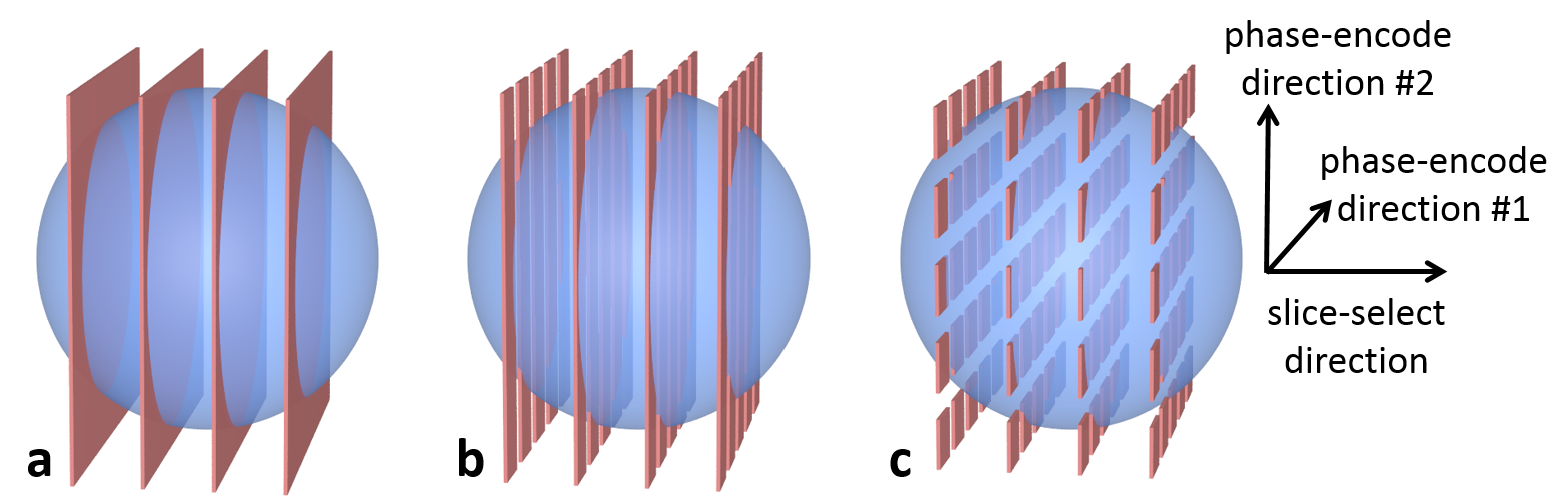
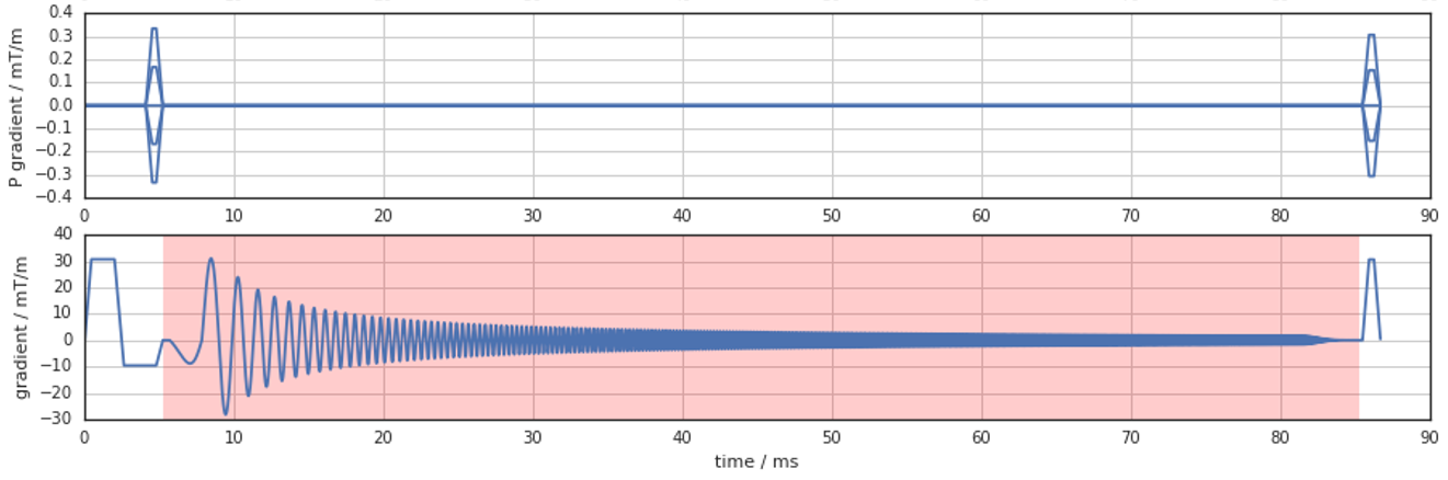
For the conventional thin slice approach2, we sequentially excite four parallel slices around the magnet's isocenter (Fig. 1a), whose spins probe the effect of a test waveform that is played after the slice selection gradient along the same direction. A slew-rate limited chirp is used as test waveform3 (lower graph of Fig. 2). From the measured phase responses, the local field at the positions of the selected slices can be determined. A reference measurement with inverted gradient is performed and subtracted for suppression of effects not related to the test waveform4, and the measurements are repeated for each gradient axis. Polynomials up to 3rd spatial order are fitted to the data to extract the 1D spatial response patterns. Relating these responses to the input waveform enables calculation of the GIRF and GMTF for different 1D spatial orders, e.g. the 0th order term ΔB0 and the direct gradient response (e.g. Gxx).
For the proposed extension of the method, phase encoding gradients are added to the sequence in one or two directions6 (upper graph of Fig. 2). Thus, each slice is partitioned into strips or rectangles (Fig. 1b,c), whose individual responses can be determined. After selection of only the signals originating from inside the phantom via thresholding, the responses are assigned to the spatial center points of the encoded regions and their spatial pattern is expanded into real-valued spherical harmonics. Now, also cross terms (e.g. Gxy and Gxz) as well as 3D higher order terms can be determined.
Measurements were performed on a Philips Ingenia 3.0 T system using a spherical water/CuSO4 phantom (T1 = 270 ms, T2 = 210 ms) with a diameter of 17 cm. Four slices with a distance of 22 mm and a thickness of 1.5 mm were acquired per gradient direction. For the presented data, only one phase encode direction was used and a high number of 65 encoding steps was chosen to increase SNR. Further scan parameters were: TE = 4 ms, TR = 4000 ms, TAQ = 80 ms, Gmax = 30 mT/m, Smax = 200 mT/m/ms, and chirp frequency range 400 Hz to 40.0 kHz. The long TR enabled interleaving acquisitions for different slices leading to a total scan time of 8 min 40 s.
Results
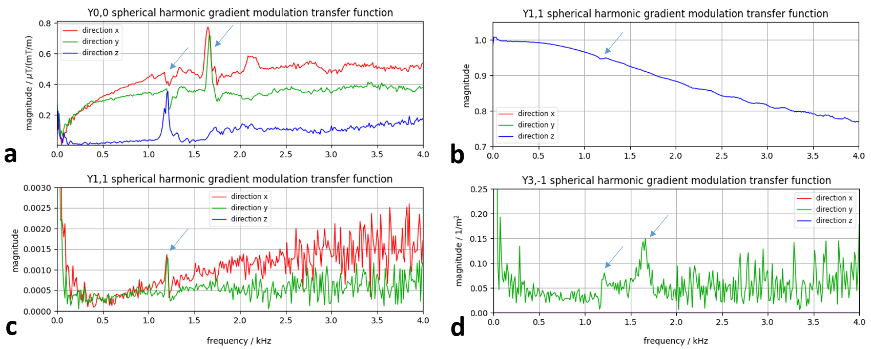
Figure 3 shows selected spherical harmonics determined from a fit to the acquired chirp data. Fig. 3a and 3b show 0th and 1st order GMTF spectra that can also be obtained using the conventional 1D method5. Phase encoding now enables the collection of perpendicular spatial information, so that linear cross terms (Fig. 3c) and higher order harmonic terms (Fig. 3d) can be determined.Discussion
The measured 0th order GMTF (Fig. 3a) mainly reflects mechanical resonances (arrows) and slight inaccuracies in system calibration, while the direct 1st order response (Fig. 3b) shows the low-pass filter characteristic of the gradient chain. Linear cross term spectra (Fig. 3c) acquired using the phase-encoded approach indicate that energy is transferred between orthogonal directions mainly at the mechanical resonance frequencies. Spatially more complex 3rd order response patterns also occur mainly close to mechanical resonances as visible at 1.2 and 1.6 kHz in the spectrum shown in Fig. 3d.
Below the lower cut-off frequency of the chirp excitation at 400 Hz, the GMTF spectra show high noise levels. To improve SNR, triangular pulses, which provide high spectral density at low frequencies, could be used in combination with the chirp pulses in the future.
Conclusion
Phantom-based gradient response characterization with phase encoding is a time-efficient method for the measurement of cross and higher order terms without the need for additional hardware. Full 3D characterization of the spatial gradient response is of interest for the characterization of new gradient coil designs, e.g. in hybrid MR systems7,8.Acknowledgements
We thank C. Stehning for providing the initial chirp GIRF software implementation.References
- Vannesjo, S. J. et al. Gradient system characterization by impulse response measurements with a dynamic field camera. Magn. Reson. Med. 69, 583–593 (2013).
- Duyn, J. H., Yang, Y., Frank, J. A. & van der Veen, J. W. Simple Correction Method for k-Space Trajectory Deviations in MRI. J. Magn. Reson. 132, 150–153 (1998).
- Addy, N. O., Wu, H. H. & Nishimura, D. G. Simple method for MR gradient system characterization and k-space trajectory estimation. Magn. Reson. Med. 68, 120–129 (2012).
- Brodsky, E. K., Klaers, J. L., Samsonov, A. A., Kijowski, R. & Block, W. F. Rapid measurement and correction of phase errors from B0 eddy currents: Impact on image quality for non-cartesian imaging. Magn. Reson. Med. 69, 509–515 (2013).
- Campbell-Washburn, A. E., Xue, H., Lederman, R. J., Faranesh, A. Z. & Hansen, M. S. Real-time distortion correction of spiral and echo planar images using the gradient system impulse response function. Magn. Reson. Med. 75, 2278–2285 (2016).
- Alley, M. T., Glover, G. H. & Pelc, N. J. Gradient characterization using a Fourier-transform technique. Magn. Reson. Med. 39, 581–587 (1998).
- Poole, M. et al. Split gradient coils for simultaneous PET-MRI. Magn. Reson. Med. 62, 1106–1111 (2009).
- Lagendijk, J. J. W., Raaymakers, B. W. & van Vulpen, M. The Magnetic Resonance Imaging–Linac System. Semin. Radiat. Oncol. 24, 207–209 (2014).
Figures