0941
Trajectory correction for a 3D-Ultrashort Echo Time (UTE) sequence using the gradient system transfer function1Department of Diagnostic and Interventional Radiology, University Hospital of Würzburg, Würzburg, Germany, 2X-Ray and Molecular Imaging Laboratory, Ostbayerische Technische Hochschule Amberg-Weiden, Weiden, Germany
Synopsis
3D-Ultrashort Echo Time (UTE) sequences with 3D-kossh ball trajectory suffer from k-space trajectory deviations and ghosting artifacts due to hardware imperfections. The gradient system transfer function (GSTF), completely characterizes the gradient system as a linear and time-invariant (LTI) system. In this study, the GSTF was measured only using standard scanner hardware and was used to correct deviated trajectories in image reconstruction. This results in diminished ghosting artifacts and improve image quality.
Purpose
In non-Cartesian imaging, non-compensated eddy currents, readout timing, amplifier errors and other system imperfections can lead to k-space deviations1. A 3D-Ultrashort Echo Time (UTE) sequence, with a 3D-koosh ball trajectory2,3 suffers from trajectory deviations which cannot be eliminated by standard trajectory correction techniques. The purpose of this work was to utilize the GSTF to correct the deviated kooshball trajectory and reduce image artifacts in image reconstruction.Methods
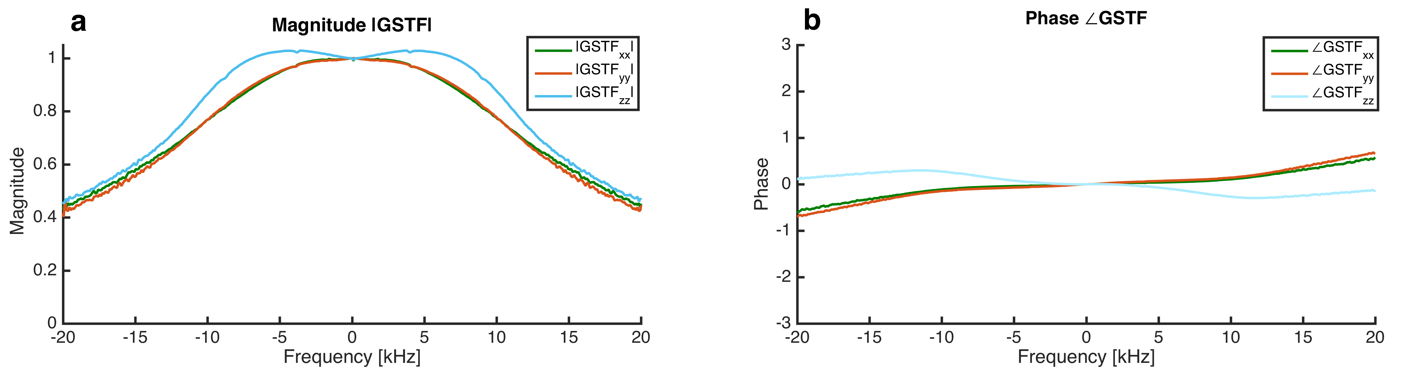
A 3D-Ultrashort Echo Time (UTE) sequence2,3 was implemented on a 3T MR system (MAGNETOM Prismafit, Siemens Healthcare, Erlangen, Germany) and measurements were performed with a 32-channel head coil in a structural phantom and in head-measurements in-vivo. The UTE pulse sequence featured a 3D-koosh ball center-out trajectory with a quasi-random sampling order. For the UTE acquisition the following parameters were applied: TE = 0.03 ms, TR = 1.49 ms, flip angle = 2°, in- plane resolution = 2.3 mm x 2.3 mm, slice thickness = 2 mm and number of spokes = 350000. A separate GSTF of the MR system for each spatial dimension was determined using triangular input gradients4,5. In a prototype sequence, 12 different input gradients (duration 100 – 320 µs, slew rate = 180 T/m/s) were played out, and the system’s response was measured in two parallel slices of a spherical phantom. The output gradient was then calculated using the difference in phase evolution between both slices. The relevant measurement parameters were set to: TR = 5.0 s, slice thickness = 3 mm, slice gap = 33 mm, flip-angle = 90°, read-out bandwidth = 100 Hz/pixel, 60 averages.
The magnitude and phase of the relevant GSTFxx, GSTFyy and GSTFzz are shown in Fig. 1. For the GSTF trajectory prediction the nominal gradient signals $$$g_{nom}(t)$$$ were corrected using GSTF information. The corrected gradient waveforms $$$g_{corr}(t)$$$ were calculated as:
$$g_{corr}(t)=\mathscr{F}^{-1}\{\mathscr{F} \{ g_{nom}(t) \} \cdot GSTF \}.$$
Images of the structural phantom and in-vivo measurements were then reconstructed using convolution gridding with the nominal trajectory and the corrected trajectory after the GSTF-information was applied to the nominal gradient waveform.
Results
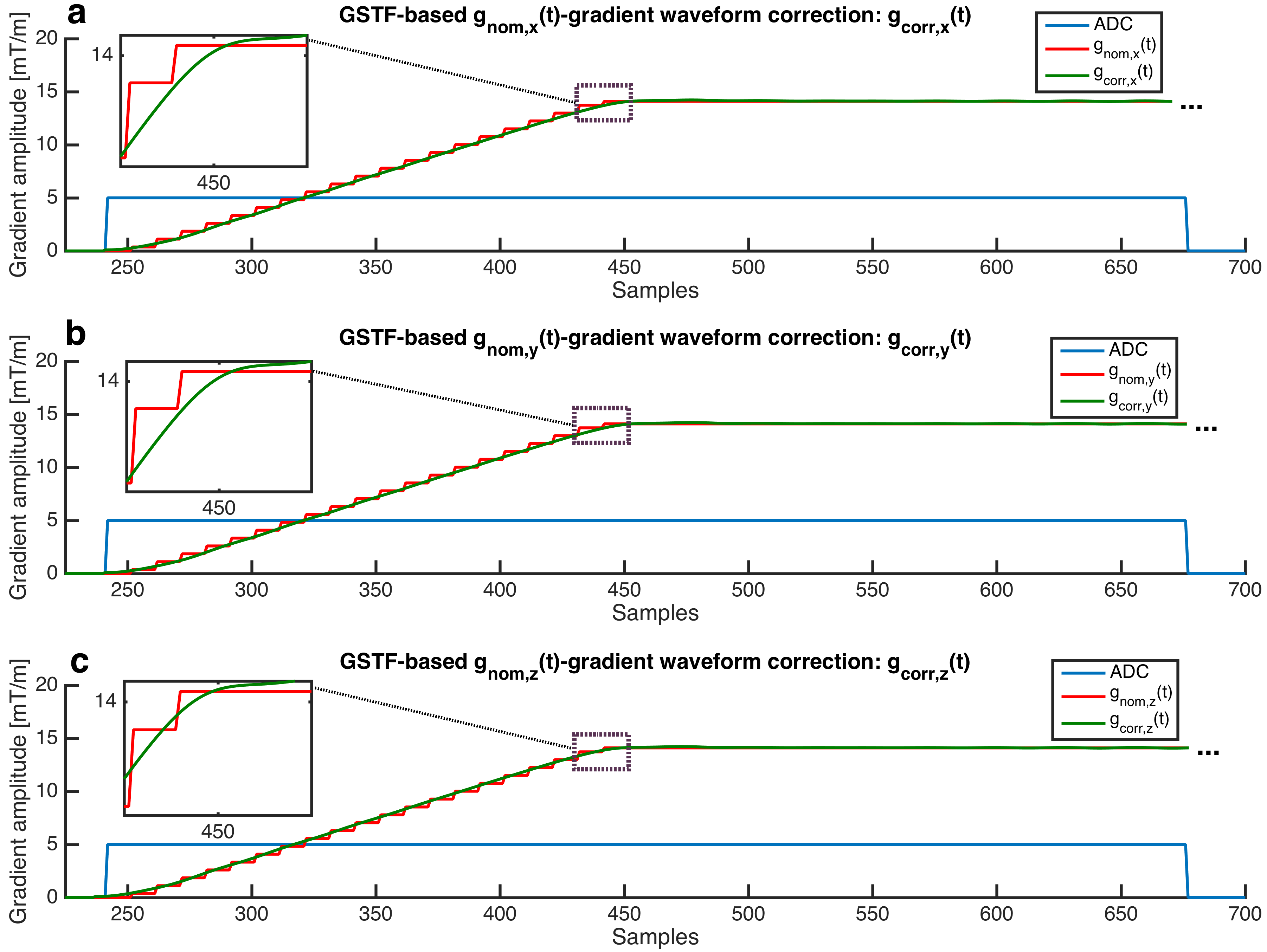
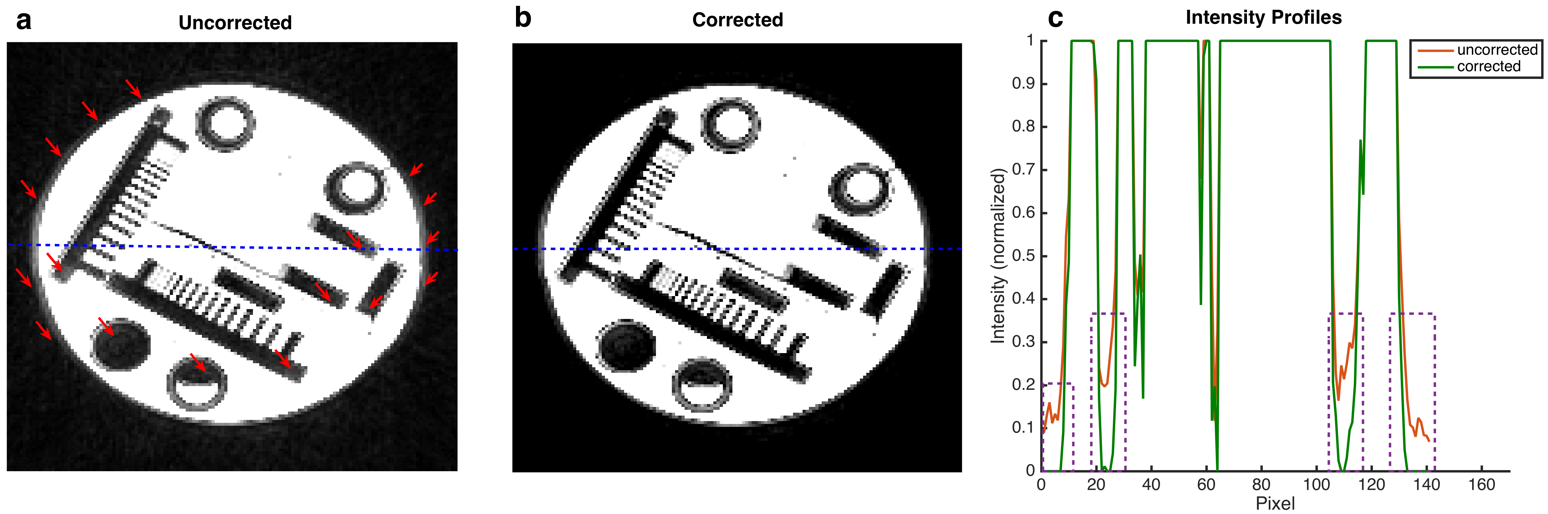
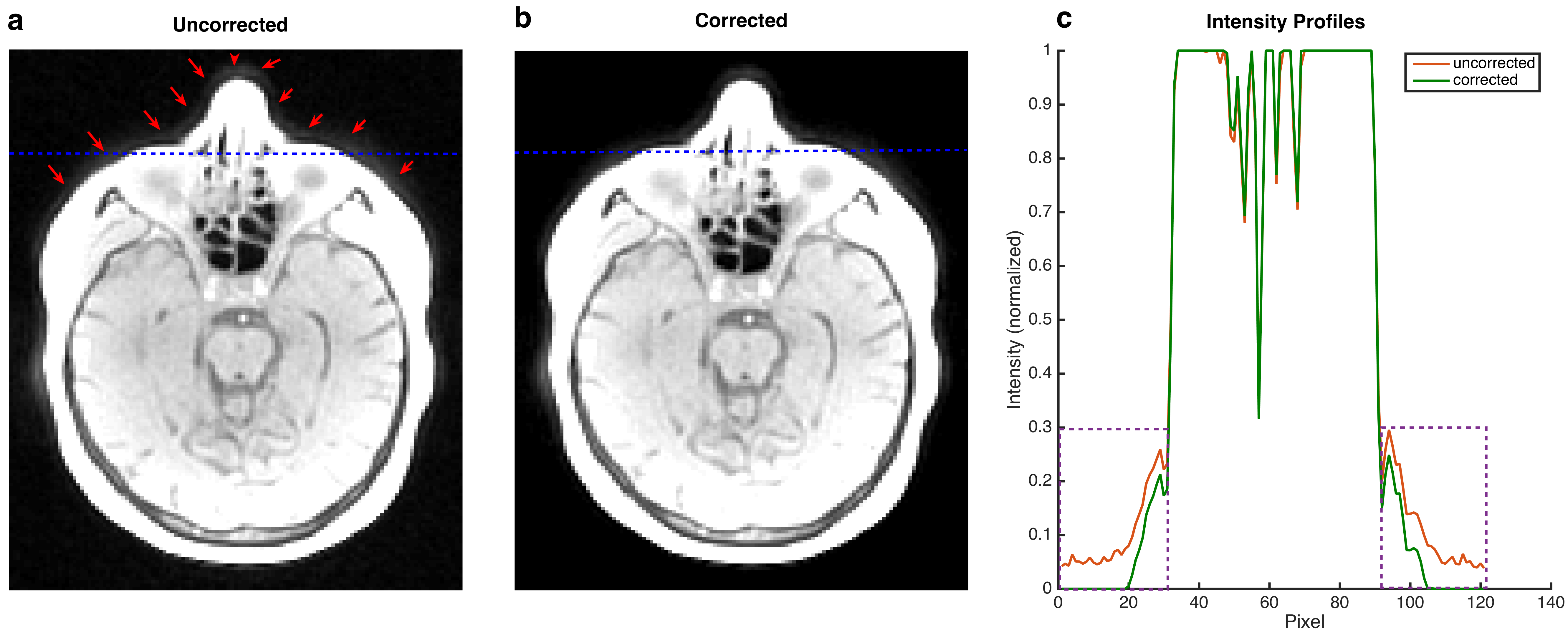
Fig. 2 shows a part of one nominal $$$g_{nom}(t)$$$ and corrected gradient waveform $$$g_{corr}(t)$$$ for all three axes. The nominal gradient on each of the three spatial dimensions has the same discrete trapezoidal waveform but different amplitudes. The correction of the x- and y-gradient is nearly the same due to the high similarity of GSTFxx and GSTFyy (see Fig. 1), while the correction of the z-gradient has a different character (see detailed view, Fig. 2). Fig. 3 shows the reconstructed phantom images (a, b), together with the intensity profile at the position of the dashed line (c). Artifacts are present if no correction is applied (Fig. 3 a, c). When considering the reduced frequency transmission rate and delay of the gradient system within a GIRF-predicted correction of the trajectories in image reconstruction, the image artifacts are suppressed (Fig. 3 b, c). The in-vivo head acquisitions are showing equivalent results: Artifacts, which are present in the image without any correction (Fig. 4 a) can be reduced by applying a GSTF-based gradient waveform correction (Fig. 4 b, c).Discussion & Conclusion
The GSTF of the MR system was determined using only standard MR hardware without special equipment such as field probes or a field camera. Its application to the gradient waveforms of a typical UTE pulse sequence corrected k-space deviations caused by hardware imperfections, such that artifacts could be diminished. In contrast to gradient measurements6,7, which would have to be carried out for all readout directions, the GSTFs have only to be acquired and can then be applied to different gradients or slice orientations.Acknowledgements
No acknowledgement found.References
1. Vannesjo SJ, Haeberlin M, Kasper L, et al. Gradient system characterization by impulse response measurements with a dynamic field camera. Magn Reson Med 2013;69:583–593.
2. Pereira LM, Wech T, Weng A, et al. Self-gated Non–Contrast-Enhanced Functional Lung (SENCEFUL) MRI for Evaluation of Endoscopic Lung Volume Reduction in Patients with Lung Emphysema. Proc. Intl. Soc. Mag. Reson. Med. 2017;25:331.
3. Pereira LM, Weng A, Wech T, et al. UTE-SENCEFUL: High resolution functional lung imaging. Magn Reson Mater Phy. 2017;30:358.
4. Campbell-Washburn AE, Xue H, Ledermann RJ, et al. Real-time distortion correction of spiral and echo planar images using the gradient system impulse response function. Magn Reson Med 2016;75:2278–2285.
5. Liu H, Matson GB. Accurate Measurement of Magnetic Resonance Imaging Gradient Characteristics. Materials (Basel). 2014;7:1–15.
6. Duyn JH, Yang Y, Frank JA, et al. Simple correction method for k-space trajectory deviations in MRI. J Magn Reson 1998;132:150–153.
7. Zhang Y, Hetherington HP, Stokely EM, et al. A novel k-space trajectory measurement technique. Magn Reson Med 1998;39:999–1004.
Figures