0890
Imaging Microscopic Background Gradient Variations in the Mouse Brain1Dept. of Radiology, New York University School of Medicine, New York, NY, United States, 2Dept. of Radiology, Johns Hopkins University School of Medicine, Baltimore, MD, United States
Synopsis
Microstructures in biological tissues can produce susceptibility related microscopic background gradient (μBG). Mapping the spatial distributions of μBG can help us infer tissue microstructure. In this study, we reported an improved diffusion MRI based method to detect μBG and evaluated the method using a phantom as well as normal and dysmyelinated mouse brains. We found that 3D spatial variations of μBG were greater in white matter tracts than in gray matter structures. The contrast based on μBG spatial variations was able to distinguish white matter tracts in normal and dysmyelinated mouse brains. The method may be used to study myelin injury.
Introduction
Background gradients due to field inhomogeneity can be found macroscopically at air tissue interfaces and microscopically between cellular compartments (1). In diffusion MRI (dMRI), background gradient may introduce a bias in quantitative measurements. Several studies have characterized the effects of background gradient on dMRI signals and described ways to reduce signal loss and distortions due to background gradients (2-4). Recent studies, however, demonstrated that dMRI can detect spatial variations of microscopic background gradient (μBG) and use the information to explore tissue microstructural organization (4-6). In this study, we designed an improved method to map μBG in wild-type mouse brains and examined its ability to detect abnormal myelination in the dysmyelinated Shiverer mouse brains.Theory
Previous reports (2,7) showed that diffusion encoding using the BGP waveform (Fig. 1) is not affected by background gradient, whereas the BGPR waveform is sensitive to background gradient. We chose to compare the BGP and BGPR (BGP/R) measurements because the two waveforms only differ in gradient polarity after the refocusing pulse, which minimizes potential biases from timing differences and eddy currents. The signal attenuations equations for BGP/R are: $$$\frac{S_{BGPR}}{S_{0}}=e^{-D( C_{ss}\cdot{\bf G_s^2}+C_{ll}\cdot{\bf G_l^2}+C_{sl}\cdot{\bf G_s}\cdot{\bf G_l})}$$$ and $$$\frac{S_{BGPR}}{S_{0}}=e^{-D( C_{ss}\cdot{\bf G_s^2}+C_{ll}\cdot{\bf G_l^2})}$$$, where SBGPR, SBGP, and S0 are the diffusion-weighted and non-diffusion-weighted signals measured. Gs and Gl are diffusion sensitizing and local background gradient vectors, D is the apparent diffusion coefficient along the direction of Gs. Css, Csl, and Cll are defined as in (2).
In a pixel with a spatial varying μBG, the ensemble average can be approximated as
$$\frac{S_{BGPR}}{S_{BGP}}={<e^{-D( C_{sl}\cdot{\bf G_s}\cdot{\bf G_l})}>} \approx {e^{-D( C_{sl}\cdot{\bf G_s}\cdot<{\bf G_l}>)}}\cdot{e^{-\frac{D^2\cdot{C_{sl}^2}\cdot{\bf G_{s}^2}\cdot{\sigma^2}}{2}}}$$
where < Gl> is the ensemble average of Gl, and σ2 is the variance of Gl along the direction of Gs. For each diffusion direction, we compared BGP/R measurement (+) with measurement along the opposite direction (-) and estimate < Gl> and σ2 using the following equations.
$$\ln(\frac{S_{BGPR}^+}{S_{BGP}^+})-\ln(\frac{S_{BGPR}^-}{S_{BGP}^-})=-2D{C_{sl}}\dot{\bf G_{s}}\dot{<\bf G_{l}>}$$
$$\ln(\frac{S_{BGPR}^+}{S_{BGP}^+})+\ln(\frac{S_{BGPR}^-}{S_{BGP}^-})=-{D^2{C_{sl}^2}\dot{\bf G_{s}^2}\dot{\bf \sigma^2}}$$
We then fitted the estimated σ2 along multiple directions (n≥6) to a tensor model to resolve the directions of maximum and minimum μBG variations.
Methods
Experiments were performed on a horizontal 7T MRI system. A phantom with tubes that contained ultrasmall superparamagnetic iron oxide (Ferraheme) suspended in agarose gel at different concentrations were used to test the BGP/R sequences with a spin echo acquisition (δ/Δ=4/5 ms, b=200-800 s/mm2). Post-mortem wildtype (n=3) and Shiverer mouse brains (n=3) were imaged using the BGP/R sequences with a single-shot EPI acquisition (TE/TR=45/2000 ms, δ/Δ=4/5 ms, 9 directions, b=300-1500 s/mm2). T2-weighted and DTI data were acquired.Results
Fig. 2 shows BGP/R signal attenuations from the phantom. In areas near the air-filled sample tube, where we expected macroscopic background gradient with small local variations, the +/- BGPR measurements were symmetric to the BGP measurements (Fig. 2A). From the gel within the tube, where we expected minimal macroscopic background gradient but strong local variations caused by superparamagnetic particles, the average of +/- BGPR measurements were no longer symmetric to the BGP measurements, suggesting that μBG variance ( σ2) was detectable (Fig. 2B), as suggested by (4).
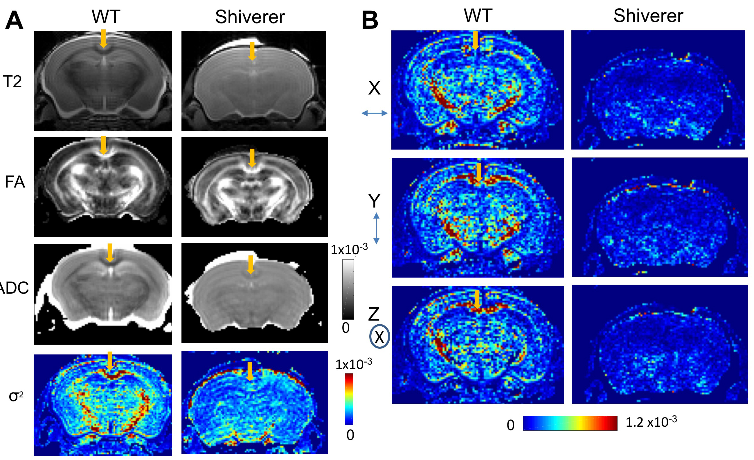
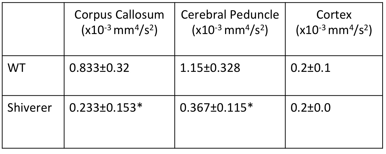
Fig. 3A shows T2-weighted, fractional anisotropy (FA), apparent diffusion coefficient (ADC) from a Shiverer mouse brain, which showed reduced white matter contrasts due to dysmyelination compared to the wild-type (WT) brains. In the μBG variance (σ2) maps, white matter structures in the WT mouse brains had significantly higher σ2 than the WT cortex and corresponding structures in the Shiverer mouse brain (Table 1). Variance maps along the x (left-right), y (dorsal-ventral), and z (rostral-caudal) axes (Fig. 3B) also showed significantly larger σ2 in the WT mouse brain than in the Shiverer mouse brain along all three axes. In the corpus callosum of the WT mouse brain, the variances along the y and z axes (perpendicular to the axons) were higher than the variance along the x (left-right) axis (parallel to the axons). The anisotropy in μBG variance likely reflected the organization of myelin sheath surrounding the axons.
Discussions and Conclusions
We have demonstrated a method to detect μBG and its spatial variation in the brain. Compared to previous methods (4-6), the BGP/R waveforms potentially allowed more sensitive detection of background gradient due to its simplicity and robustness. In addition, our method can estimate μBG and especially its 3D variance as a full rank tensor, which has not been achieved before. The 3D variance of μBG reflects the underlying microstructure organization. The contrast provided by our method is a unique addition to existing dMRI contrasts and may be used to sensitively detect myelin injury.Acknowledgements
No acknowledgement found.References
1. Reichenbach JR, Venkatesan R, Yablonskiy DA, Thompson MR, Lai S, Haacke EM. Theory and application of static field inhomogeneity effects in gradient‐echo imaging. Journal of Magnetic Resonance Imaging 1997;7(2);266-279.
2. Hong X, Dixon T. Measuring diffusion in inhomogeneous systems in imaging mode using antisymmetric sensitizing gradients. Journal of Magnetic Resonance 1992;99:561–570.
3. Jara H, Wehrli F. Determination of Background Gradients with Diffusion MR Imaging. Journal of Magnetic Resonance Imaging 1994;4:787–797.
4. Zhong J, Kennan R, Gore J. Effects of susceptibility variations on NMR measurements of diffusion. Journal of Magnetic Resonance (1969) 1991;95:267–280
5. Han SH, Song YK, Cho FH, Ryu, Cho, Song Y-Q, Cho. Magnetic field anisotropy based MR tractography. Journal of Magnetic Resonance 2011;212:386–393.
6. Álvarez G, Shemesh N, Frydman L. Internal gradient distributions: A susceptibility-derived tensor delivering morphologies by magnetic resonance. Scientific Reports 2017;7:3311.
7. Trudeau, Dixon, Hawkins. The effect of inhomogeneous sample susceptibility on measured diffusion anisotropy using NMR imaging. 1995; 108(1):22-30
Figures