0875
Visual temporal frequency preference shows a distinct cortical architecture using fMRI1National Institute of Mental Health, National Institutes of Health, Bethesda, MD, United States
Synopsis
The functional architecture of temporal frequency preference of human visual system is not well characterized. We collected fMRI data with visual stimuli varying flicker frequency from 1 to 40 Hz. Using model fit and K-means clustering on frequency tuning curve we were able to show evidence for a temporal frequency specific architecture of visual system.
Introduction
Temporal frequency is a fundamental attribute of visual stimuli. Frequency sensitivity has been studied in multiple areas of the visual system, including lateral geniculate nucleus, superior colliculus, primary visual cortex and high-level visual areas1–4. But these studies typically examine frequencies under 20 Hz and have not attempted to map preferred temporal frequency across many visual areas. In this study, we aimed to generate a temporal frequency preference map for the human visual system, and ask if this temporal frequency selectivity is organized into a functional architecture.Methods
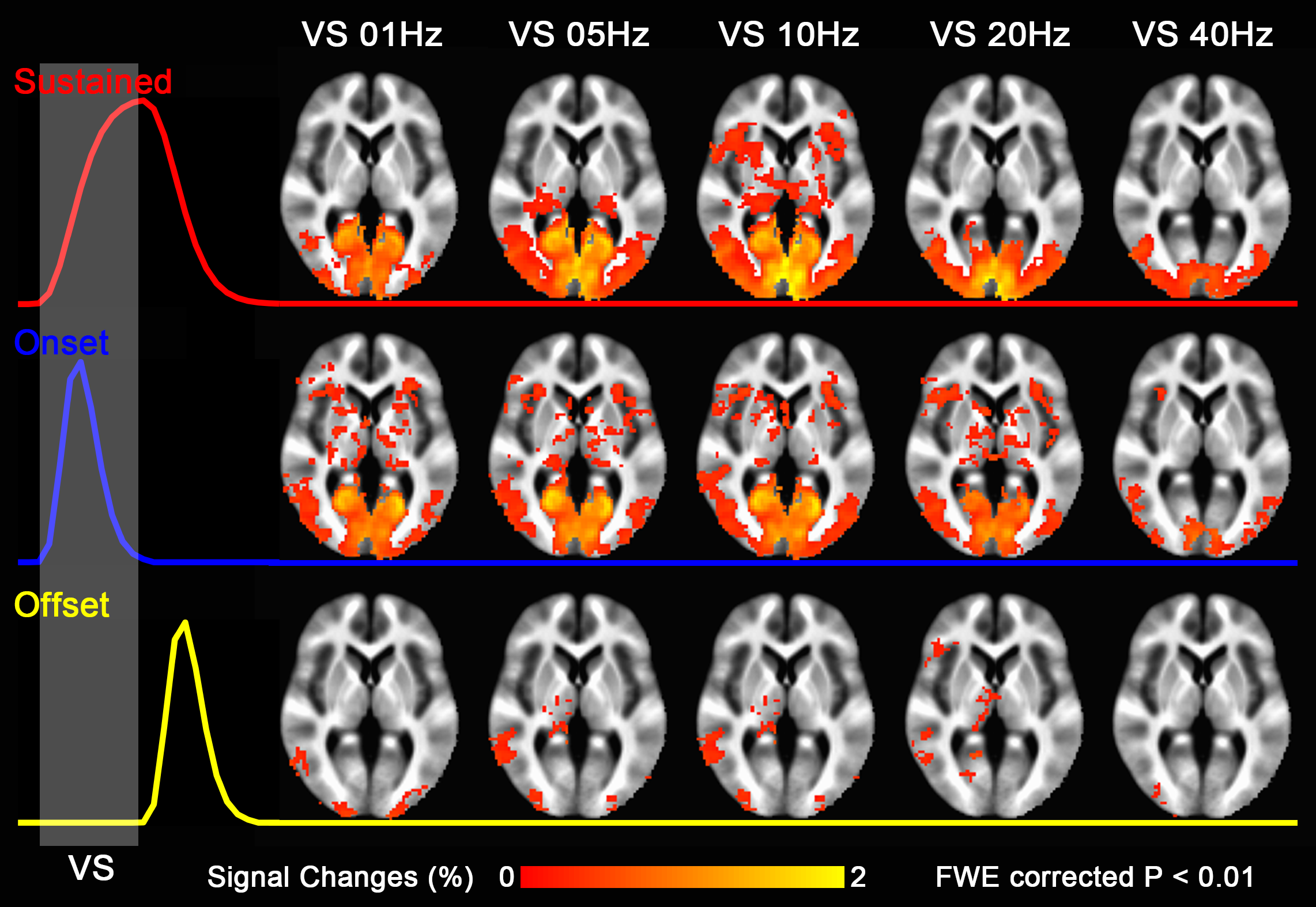
Twenty right-handed subjects (ten males/ten females; aged 18-50, mean age 26.5) were scanned on a 3T system (Siemens Prisma). A block design was utilized (10 s ON/20.6 s fixation). During the ON segment, visual full-field stimulation at one of five temporal frequencies (1 Hz, 5Hz, 10 Hz, 20 Hz and 40 Hz) was applied, alternating the whole screen (BOLDscreen 32 LCD) from black to white. Frequency order was randomized. Simultaneous multi-slice (SMS) EPI was used with TR/TE = 1700/28 ms, matrix 90×90, 2.5mm isotropic voxels, 52 slices, SMS factor = 2, no in-plane acceleration. Statistical analyses were conducted with AFNI using an onset + sustained + offset BOLD response model5,6. For active voxels (cluster-based thresholding p < 0.01), the sustained BOLD signal changes across temporal frequencies were fitted with a difference of exponentials function7,8. The peak frequency was used to display tuning maps only if the correlation coefficient of the fitting was larger than 0.32. BOLD signal changes at each frequency were also inputted to the K-Means clustering algorithm to group areas according to the similarity of their response across frequencies.Results and discussion
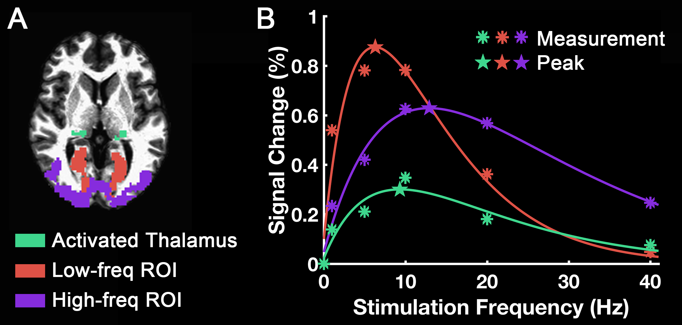
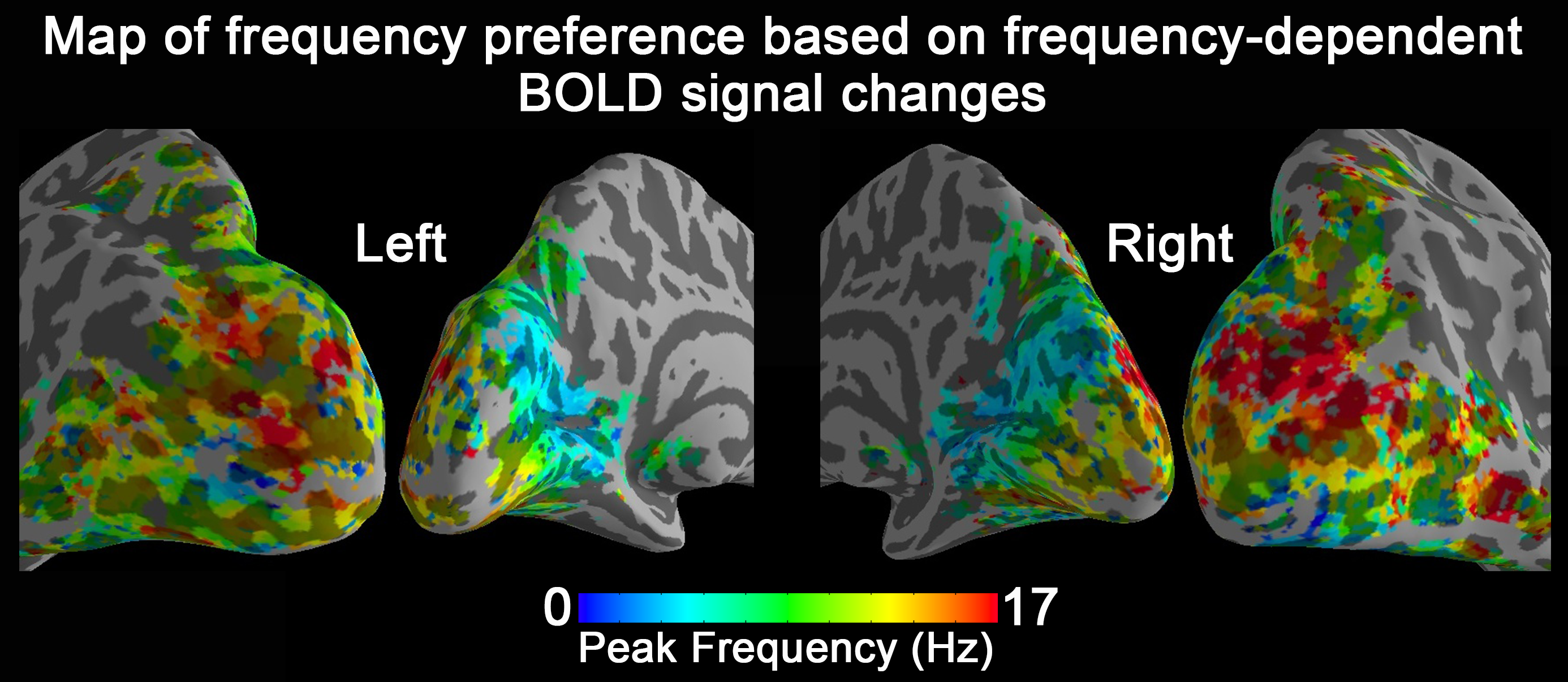
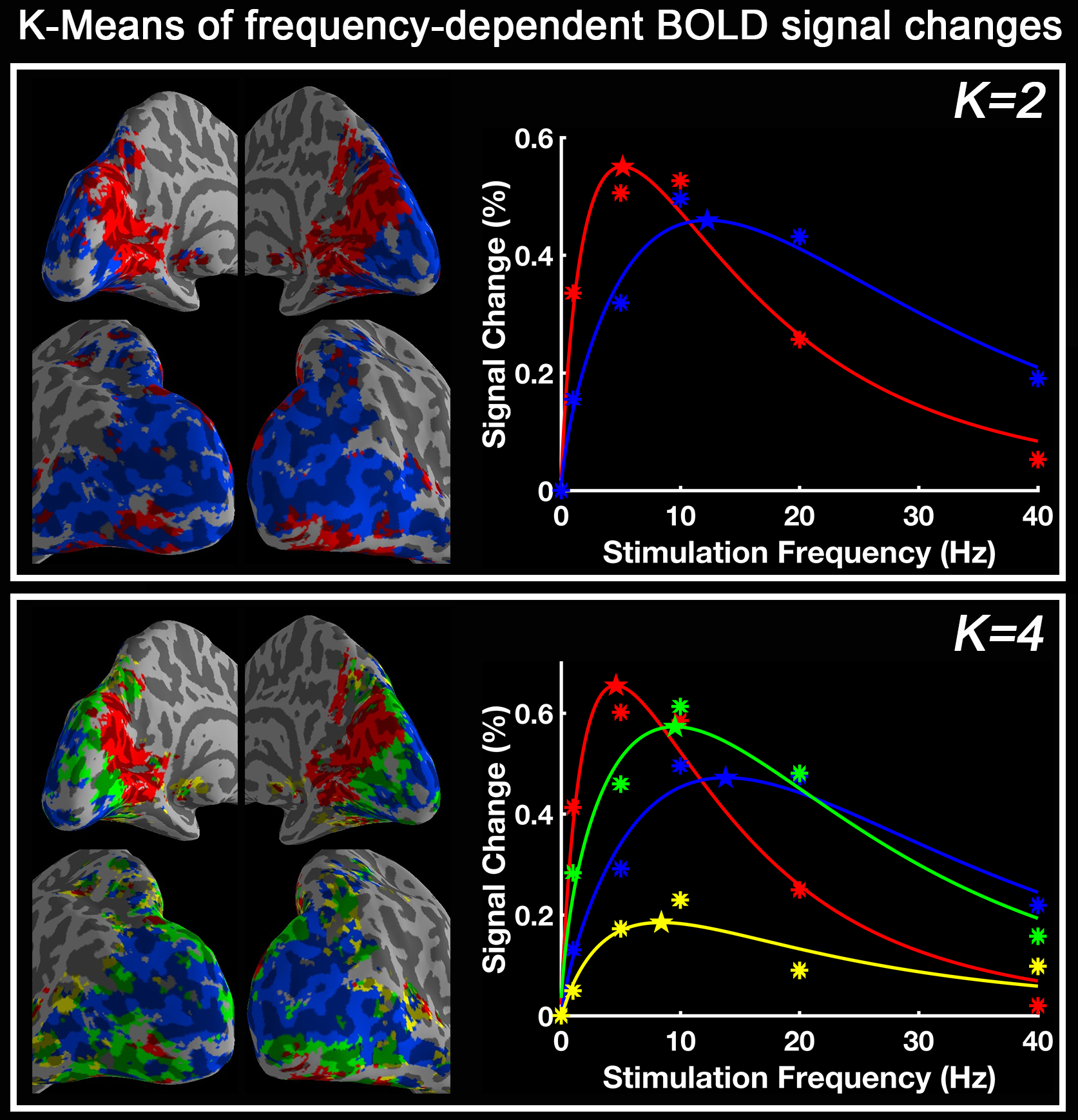
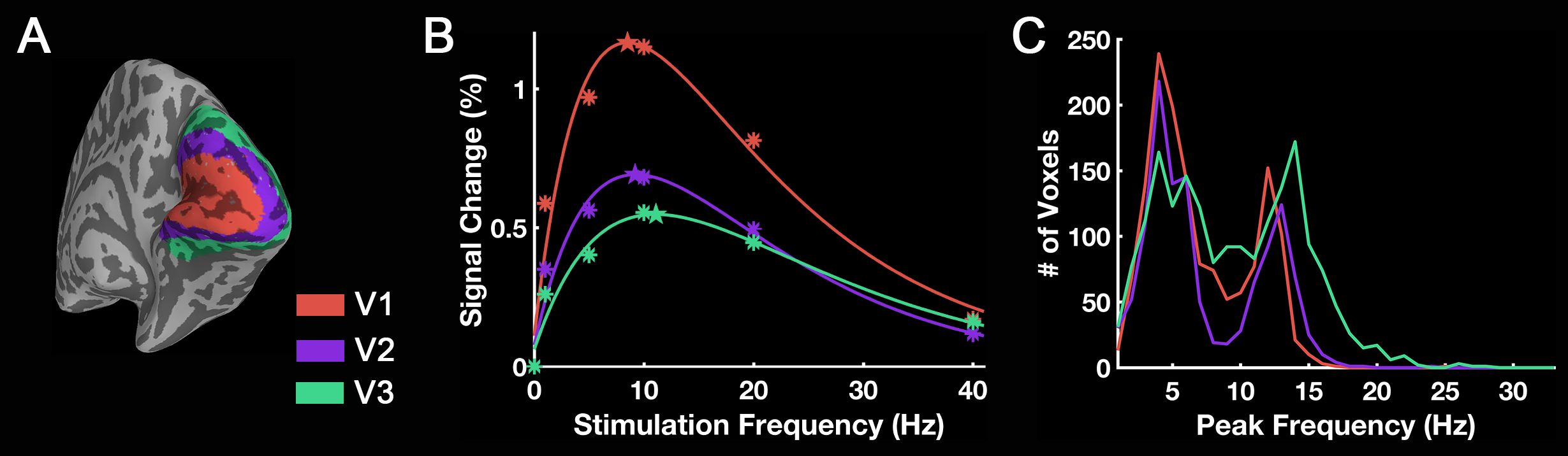
Group-level activation maps for the sustained, onset and offset BOLD response are shown in Fig. 1. Frequency-dependent spatial pattern changes are most obvious from the sustained responses, especially when comparing activation maps between 01 Hz and 40 Hz stimuli. Based on the activation map of the sustained responses, we defined three regions-of-interest (ROI) as in Fig. 2A: (1) Low frequency ROI, regions activated by 1 Hz stimuli and restricted to the calcarine sulcus; (2) High frequency ROI, occipital regions activated by 40 Hz stimuli outside the calcarine region; (3) Activated thalamic regions. The mean signal changes from these three ROIs were extracted and averaged across subjects, and plotted as a function of stimulation frequency (Fig. 2B). The signal changes vs. temporal frequencies were fitted with a difference of exponentials function and the peak frequency of the fitting curve was extracted. Then we applied this model fit to every voxel inside the visual activated areas and displayed the voxel-wise peak frequency as Fig. 3. In this tuning map, we can observe how calcarine sulcus is tuned to the lowest frequencies. When moving from the anterior to the posterior calcarine, the preferred frequency increases. Lateral occipital areas show a preference for the highest flickering frequency. In addition to model fit, we also applied K-means to decompose visual areas according to their temporal frequency response (Fig. 4). For k=2, visual areas were segmented into low and high frequency clusters. The cluster distributions of k=4 suggests a clear peak frequency increasing trend from anterior to posterior calcarine and then to lateral occipital areas. Frequency tuning curves for V1, V2 and V3 (based on a visual template9 from Benson et al. (2014)) are shown in Fig. 5B; while voxel counts tuned to the different frequencies in these three regions are shown in Fig. 5C. The mean BOLD response of V1, V2 and V3 all peaked at about 8-11 Hz, which is consistent with previous visual functional imaging researches3,10. However, most voxels in these visual areas have peak frequency of either 4 Hz or 12-14 Hz.Conclusions
The human visual areas could be arranged into several clusters, each comprising a group of areas that share a common frequency tuning response. There is a clear increasing trend of preferred temporal frequency from anterior to posterior calcarine and then to lateral occipital cortex.Acknowledgements
No acknowledgement found.References
1. Orban G a, Kennedy H, Maes H. Response to movement of neurons in areas 17 and 18 of the cat: velocity sensitivity. J Neurophysiol. 1981;45(6):1059-1073.
2. Yen CCC, Fukuda M, Kim SG. BOLD responses to different temporal frequency stimuli in the lateral geniculate nucleus and visual cortex: Insights into the neural basis of fMRI. Neuroimage. 2011;58(1):82-90. doi:10.1016/j.neuroimage.2011.06.022.
3. Singh KD, Smith AT, Greenlee MW. Spatiotemporal Frequency and Direction Sensitivities of Human Visual Areas Measured Using fMRI. Neuroimage. 2000;12(5):550-564. doi:10.1006/nimg.2000.0642.
4. Van Camp N. Light Stimulus Frequency Dependence of Activity in the Rat Visual System as Studied With High-Resolution BOLD fMRI. J Neurophysiol. 2006;95(5):3164-3170. doi:10.1152/jn.00400.2005.
5. Uludaǧ K. Transient and sustained BOLD responses to sustained visual stimulation. Magn Reson Imaging. 2008;26(7):863-869. doi:10.1016/j.mri.2008.01.049.
6. Gonzalez-Castillo J, Hoy CW, Handwerker DA, et al. Task dependence, tissue specificity, and spatial distribution of widespread activations in large single-subject functional MRI datasets at 7T. Cereb Cortex. 2015;25(12):4667-4677. doi:10.1093/cercor/bhu148.
7. Hawken MJ, Shapley RM, Grosof DH. Temporal-frequency selectivity in monkey visual cortex. Vis Neurosci. 1996;13:477-492. doi:10.1017/S0952523800008154.
8. Gegenfurtner KR, Kiper DC, Levitt JB. Functional Properties of Neurons in Macaque Area V3. J Neurophysiol Publ. 1997;77(4):1906-1923.
9. Benson NC, Butt OH, Brainard DH, Aguirre GK. Correction of Distortion in Flattened Representations of the Cortical Surface Allows Prediction of V1-V3 Functional Organization from Anatomy. PLoS Comput Biol. 2014;10(3). doi:10.1371/journal.pcbi.1003538.
10. Fox PT, Raichle ME. Stimulus rate dependence of regional cerebral blood flow in human striate cortex, demonstrated by positron emission tomography. J Neurophysiol. 1984;51(5):1109-1120.
Figures