0874
Using measured Haemodynamic Response Functions in Population Receptive Field mapping at 7 T1SPMIC, University of Nottingham, Nottingham, United Kingdom, 2University of Nottingham, Nottingham, United Kingdom
Synopsis
In order to combat overfitting in computational encoding models, one method is to reduce the number of fit parameters. In population receptive field (pRF) mapping, a haemodynamic response function (HRF) is parameterized from the fMRI timeseries, and this may inflate model fits (r2). Here, we show that measured HRF estimates from a brief set of separate HRF measurement scans can be included in the pRF fitting procedure, reducing the degrees of freedom. We show that model fits between our “HRF-informed” pRF and the traditional fitted HRFs are comparable, suggesting that this method is more representative of the ground truth.
Purpose
Population receptive field (pRF) mapping provides a powerful framework for linking the tuning properties of neurons in different cortical areas regions with measured functional MRI responses1. This method also allows for estimation of the haemodynamic response function (HRF). However, this requires up to 8 parameters in the pRF model fit (5 parameters to account for differences in HRF shape). Here, we perform voxel-wise measurements of the HRF in human early visual cortex (V1-V3) at 7T and use them to inform the pRF fitting fitting of pRF maps.Methods
fMRI data were acquired on a 7T Philips Achieva scanner using a 32-channel receive coil. Each session consisted of one scan to determine HRF shape (multiband factor 2, TR 1s, 330 dynamics), and four scans to measure pRFs (TR 2s, 126 dynamics each). Other acquisition parameters: GE-EPI BOLD, TE 25ms, (1.5mm)3 resolution, 30 slices. High-resolution Phase Sensitive Inversion Recovery (PSIR) (0.3x0.3x1mm3) and T2*-weighted (0.5x0.5x1.5mm3) scans were also acquired for co-registration and vein-masking of the functional data.
The experiment comprised of 1) HRF measurement: 5s full-field flashing-checkerboard stimulus followed by 50s fixation (mid-grey background), 6 repeats; 2) pRF mapping: visual stimuli commonly used for retinotopic mapping - rotating wedges and drifting bar apertures of high-contrast checkerboards (forward/reverse directions). Each stimulation cycle lasted 24s (10 repeats per scan). In one session, an additional HRF measurement scan was acquired with a 1s visual stimulus (54s fixation).
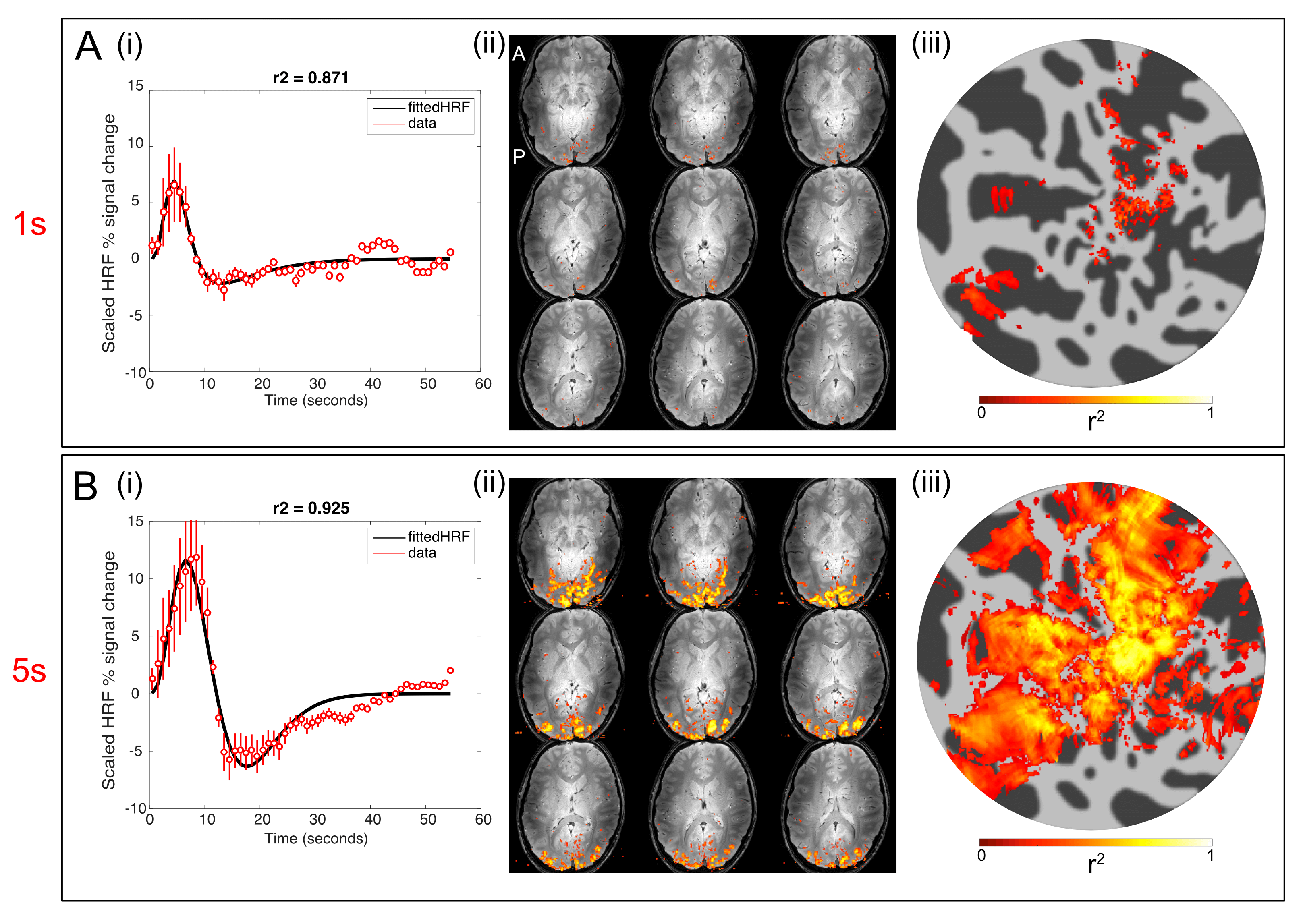
HRF Measurement: For the 1s and 5s HRF datasets, voxel-wise measured HRFs were calculated by averaging across repeats. A GLM analysis was also performed to identify active responses to each stimulus duration.
pRF Mapping: The pRF data were analyzed using standard retinotopic2 and pRF mapping1 methods. The pRF was assumed to have 2D-Gaussian profile (parameterized by [x0, y0, σ]) and overlapped with the stimulus description at each time-point to produce a predicted pRF response. This pRF response was then convolved with a HRF model (5 parameters) to produce a predicted fMRI response. The best-fit parameters for the fMRI timeseries at every voxel were estimated by nonlinear least squares3. Additionally, we input the measured 1s and 5s HRFs into the pRF model, bypassing the HRF fitting within the pRF analysis.
For visualization, all parameter maps from both the pRF and HRF analyses were superimposed on cortical surfaces derived using FreeSurfer.4,5
Results
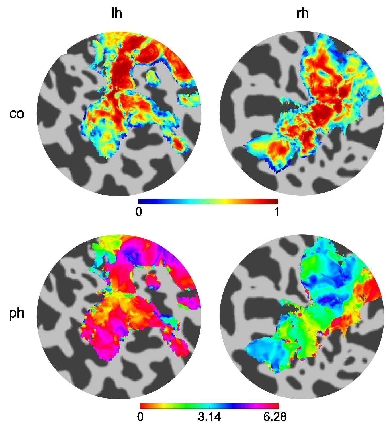
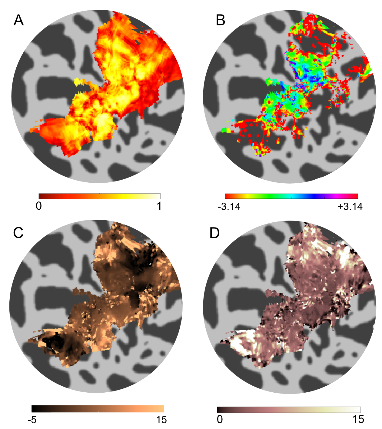
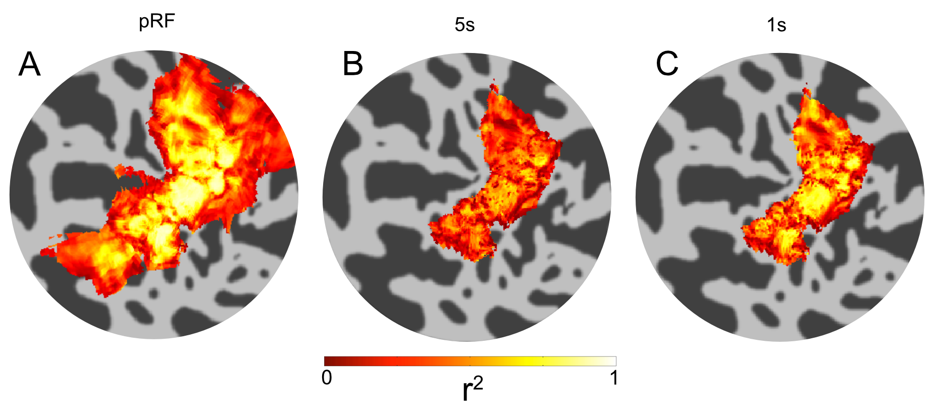
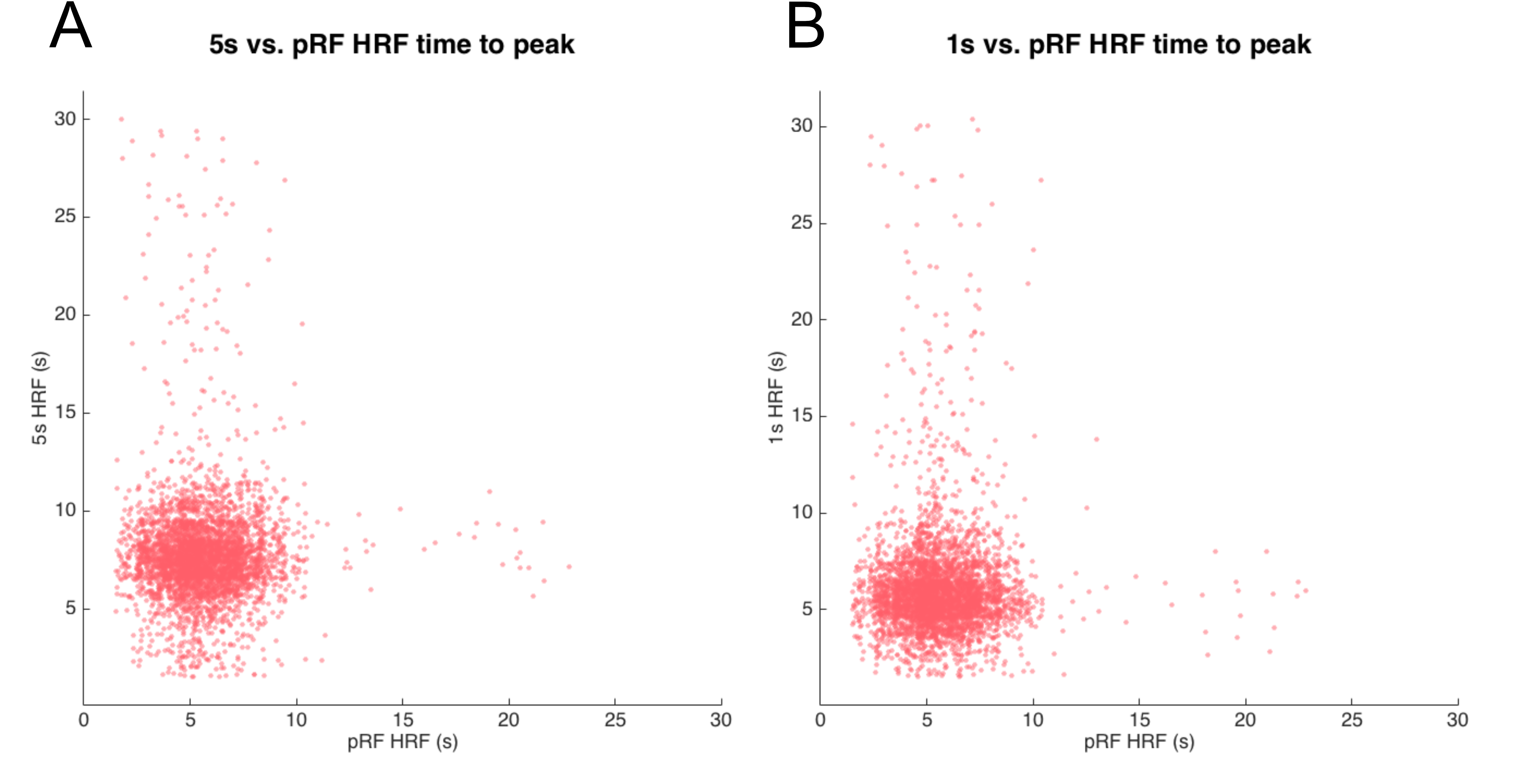
Figure 1 shows the results of the GLM analysis of the 1s and 5s visual stimulation and associated HRFs. Figure 2 shows example coherence and phase retinotopy maps. Figure 3 shows pRF parameter maps from the 8 parameter (2D Gaussian+HRF) model fit. Both coherence (retinotopy) and pRF fits (r²) were strong: for the individual pRF scans, at least 37% of voxels achieved r²>0.5, with the mean of the maximum r² = 0.93 (across four pRF scans). Figure 4 shows the results of inputting the 1s and 5s measured HRFs into the pRF model. It can be seen that the r² values for the 1s HRFs are greater than the 5s HRFs (more voxels with r²>0.5 (42% vs. 22%). Figure 5 compares the pRF-fitted HRF parameters with the 1s and 5s measured HRF responses, specifically for the time-to-peak (TTP). Note the 1s measured data shows a number of voxels with late TTPs; these are not accurately fit by the 8 parameter pRF model.Discussion
We show that inputting a measured 1s HRF into the pRF model produces similar r² fits to the pRF analysis, with the advantage of reducing the degrees of freedom. In the visual domain, r² values using the pRF with a 2D Gaussian (with HRF parameters) are high, as BOLD responses are high and hence the pRF is not SNR-limited. However, when using the pRF model in the somatosensory cortex, SNR is considerably lower, leading to high variability in the HRF model fit. Utilising subject-specific, voxel-wise HRFs in the model, as validated here, should improve the reliability of the model fit and allow a 3 parameter pRF model to be used. It is seen in this data that there are a wide range of HRF shapes (Figure 5) with later TTPs not well fit by the pRF. In further work, we will assess deconvolving the 5s HRF to extract a 1s “deconvolved” HRF; this should provide a higher SNR HRF than a 1s “measured” HRF.Conclusion
We demonstrate that a measured HRF can be used in pRF analysis in the visual cortex. In the future, this method will be assessed in other sensory domains, such as the somatosensory cortex, where fMRI responses have lower SNR, to improve the pRF fitting procedure.Acknowledgements
This work was funded by an MRC grant (MR/M022722/1).References
- Dumoulin, SO, et al. NeuroImage. 2008;39(2):647-660.
- Engel, SA, et al. Cerebral Cortex. 1997; 7(2):181-192.
- Nelder, JA, et al. The Computer Journal. 1965;308-313.
- Dale, AM, et al. NeuroImage. 1999;9:179-194.
- Fischl, B, et al. NeuroImage. 1999;9:195-207.
Figures