0835
Regularized Second-order Dynamic Shimming1Wellcome Centre for Integrative Neuroimaging, FMRIB, University of Oxford, Oxford, United Kingdom
Synopsis
The implementation of dynamic shimming relies on determining robust and accurate shim currents. This work presents a novel, analytical, and fully automated regularized shim determination technique to solve ill-conditioned least-square problems and regularize current constraint challenges for dynamic shimming applications. The method is based on the Tikhonov regularization whereby the L-curve method is utilized to search for an optimal shim solution. The method improves shim current use efficiency and conditioning of the shim determination problem, outperforming the truncated singular value decomposition regularization based least-square method.
Purpose
This work presents a novel and fully automated shim optimization algorithm for dynamic shimming. The technique simultaneously addresses fixed hardware constraints and improves the conditioning of the shim calculation by tunable regularization.Introduction
Dynamic shimming can improve B0 field homogeneity in regions with strong local field distortion.1 However, as the shim volumes get smaller, robust calculation of optimal shim settings gets harder. Partly, this is because small volumes within regions of large field distortion are more likely to run into current constraints of the shim amplifiers. Smaller volumes also make the optimization problem increasingly ill-conditioned, and thereby more susceptible to measurement noise. Additionally, there is a desire to keep shim currents low in order to reduce eddy currents and heating.
Conventional shim optimization techniques arrive at permissible shim settings with a constrained least-square linear approach. This, however, does not include regularization to reduce current amplitudes and minimize the impact of measurement errors. Previous studies have investigated using truncated singular value decomposition to enforce hardware constraints via variable regularization.2,3 For low-order shim systems, however, limited singular values are available. Therefore, truncation of singular values causes round-off errors, often leading to over-regularization.
To balance the need for regularization with the task of minimizing field inhomogeneity, we propose a shim optimization based on Tikhonov regularization in conjunction with an automated search for optimal regularization parameters using the L-curve method (Tikh-L).4
Materials and Methods
The experiments were performed on a 7T MRI scanner (Siemens Healthineers, Germany), equipped with second-order shim coils driven by external amplifiers (RRI, MA, USA). Exponential pre-emphasis was implemented on all shim channels. Dynamic shimming was performed by updating both gradients and second-order shims on a slice-by-slice basis.
The Tikh-L method is summarized in Fig. 1.
1. Calculate multiple sets of shim solutions using Tikhonov regularization with a range of regularization parameters.
2. Find solutions that lie within the dual boundaries of (1) shim current limits and (2) standard deviation constraints (<1% of an unconstrained pseudoinverse solution) to avoid over-regularization.
3. (a) If solutions exist within the boundaries, use the L-curve method to determine the optimal trade-off between the current norm and residual field inhomogeneity. (b) If no solutions exist fulfilling both boundary conditions, pick the solution yielding lowest residual standard deviation within the shim current constraints.
The performance of the Tikh-L method was evaluated compared to: (1) Unconstrained pseudoinverse, as a benchmark for the ideally achievable shimming quality; (2) A Matlab-embedded constrained least-square method with hardware constraints (LSQlin); (3) TSVD with hardware constraints (TSVD-H).
Simulations were performed on a field map database consisting of 143 whole-brain field maps from different subjects acquired using a gradient echo (GRE) field mapping sequence (2mm isotropic). For experimental evaluation, field mapping was conducted on a healthy volunteer without shimming, and with slice-wise shimming calculated with the different optimization algorithms. Echo-planar images (2mm iso-tropic, TE=28ms, PAT2, echo-spacing=0.72ms) were used to evaluate distortion and dropout.
Results
The scatter plots in Fig. 2 compare simulation results using LSQlin, TSVD-H and Tikh-L in two scenarios: shim determination (a) without and (b) with hitting current constraints. In scenario (a), Tikh-L reduces the solution norm without evidently degrading the attainable B0 field standard deviation. In scenario (b), Tikh-L yields a comparable reduction in the solution norm, while delivering better shim quality than TSVD-H. The LSQlin, TSVD-H and Tikh-L methods provide an average solution norm reduction of 27%, 74% and 52% and standard deviation degradation by 0.7Hz, 4.3Hz and 1.4Hz, respectively as compared to the unconstrained pseudoinverse. The Tikh-L did not increase the computation time compared to the other methods.
The experimental results on one example subject, as shown in Fig. 3, confirm the simulation results. The proposed Tikh-L method shows reduced solution norm and improved conditioning across different slices, especially for slices with small ROIs, as in the upper and lower parts of the brain. Fig. 4 demonstrates that Tikh-L yields comparable shimming results as LSQlin and sometimes outperforms TSVD-H - reflected in the EPI images located in the brainstem.
Discussion
Whilst LSQlin achieves the lowest residual B0 standard deviation numerically, this comes at a cost of high shim current amplitude and does not translate to better shimming in practice. The regularization-based methods trade some slight standard deviation for the much-improved current use efficiency and conditioning of least-square problems. The Tikh-L provides more degrees of freedom in regularisation than TSVD and allows for more flexible control on shimming results.
Conclusions
We demonstrated that the proposed Tikh-L technique produces satisfactory residual field homogeneity, while simultaneously improving the efficiency of the shim current use and conditioning of the least-squares problem.
Acknowledgements
Financial support was received from the Medical Research Council, the Dunhill Medical Trust, and the European Union’s Horizon 2020 research and innovation programme under the Marie Sklodowska-Curie grant 659263. We are grateful for support in the form of hardware loan and technical support from Andrew Dewdney, Siemens Healthineers.
References
1. Juchem C, Nixon TW, Diduch P, et al. Dynamic shimming of the human brain at 7 T. Concepts in Magnetic Resonance Part B: Magnetic Resonance Engineering. 2010;37(3):116-28.
2. Kim DH, Adalsteinsson E, et al. Regularized higher‐order in vivo shimming. Magnetic Resonance in Medicine. 2002;48(4):715-22.
3. Nassirpour S, et al. A comparison of optimization algorithms for localized in vivo B0 shimming. Magnetic Resonance in Medicine. 2017.
4. Hansen PC, O’Leary DP. The use of the L-curve in the regularization of discrete ill-posed problems. SIAM Journal on Scientific Computing. 1993;14(6):1487-503.
Figures
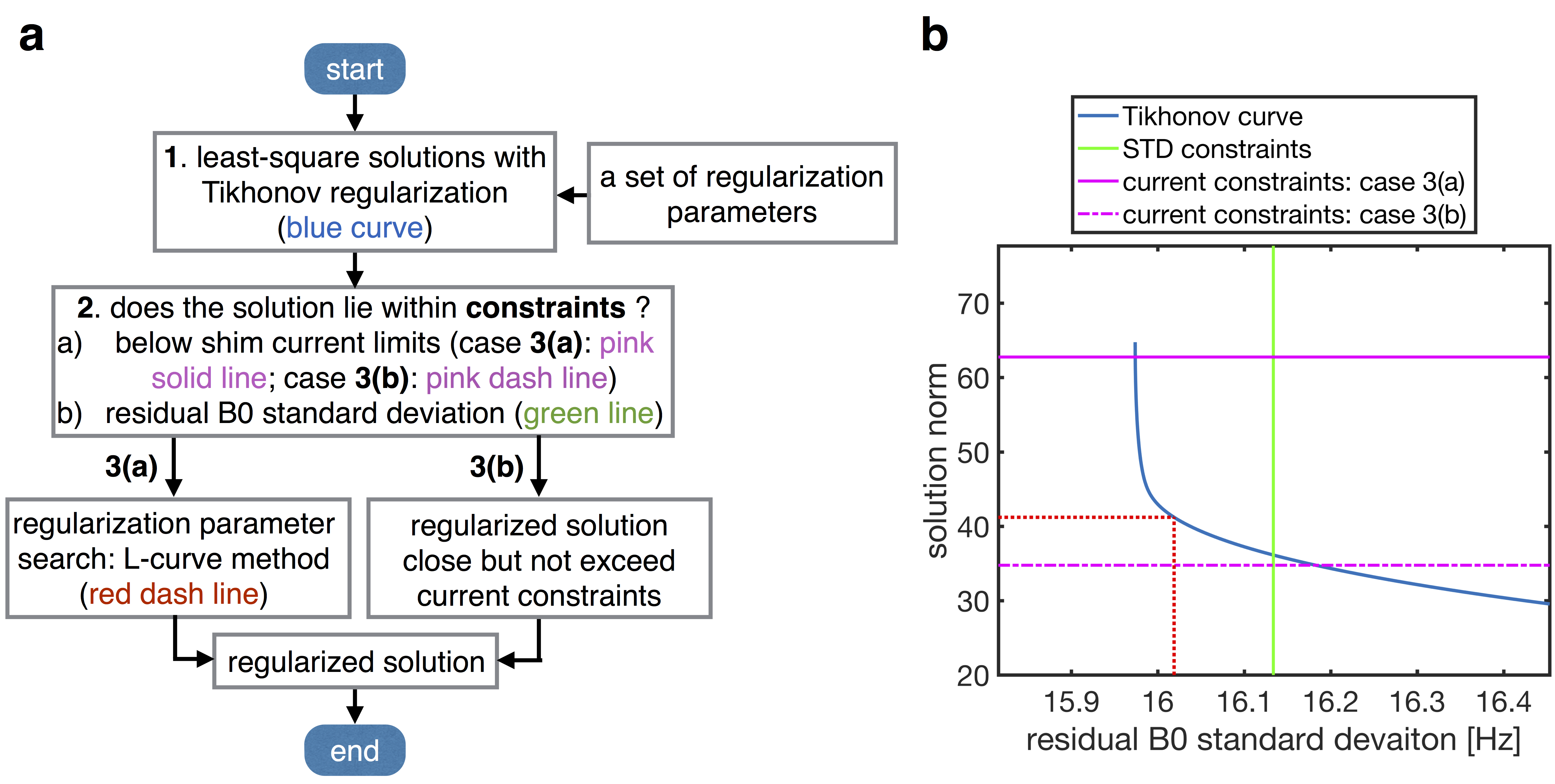
Fig. 1: Flow chart (a) and schematic example (b) of shim determination procedure of the proposed Tikh-L method. The optimal shim solution (red dashed line) is determined from a range of Tikhonov regularized solutions (blue line with a characteristic L shape) using the L-curve method along with dual constraints on the solution norm (pink solid or dashed line) and residual B0 field standard deviation (green line).
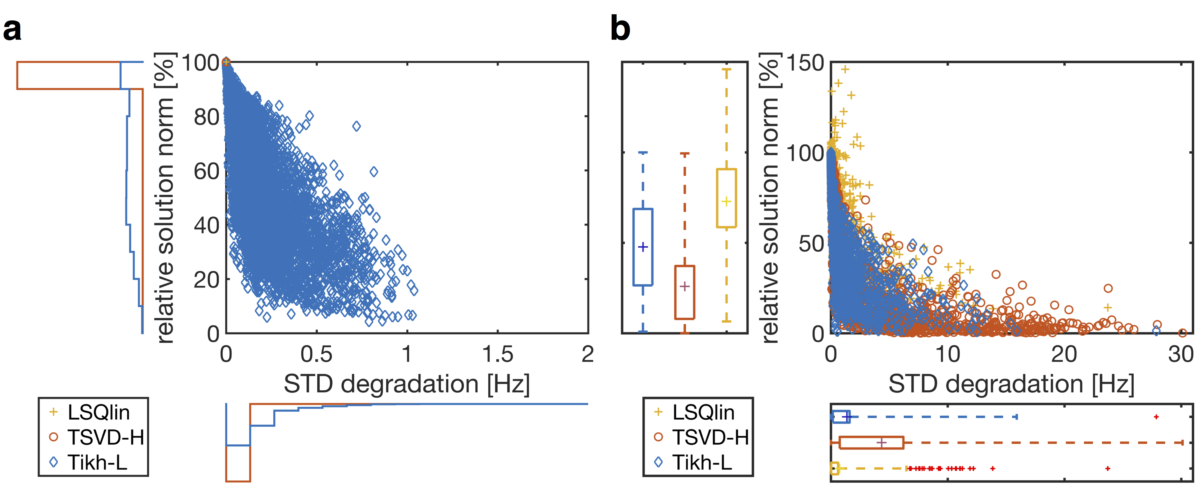
Fig. 2: Comparison of simulated shimming performance with the LSQlin (yellow), TSVD-H (red), and Tikh-L (blue) methods for each slice across all subjects in the database. The scatter plot in (a) indicates the relative solution norm reduction, along with the relative increase in the residual field standard deviation as compared to the unconstrained pseudoinverse, on slices that do not hit current constraints. The scatter plot in (b) indicates results on slices that do run into current limits. The corresponding distributions are shown separately in the histograms and boxplots.
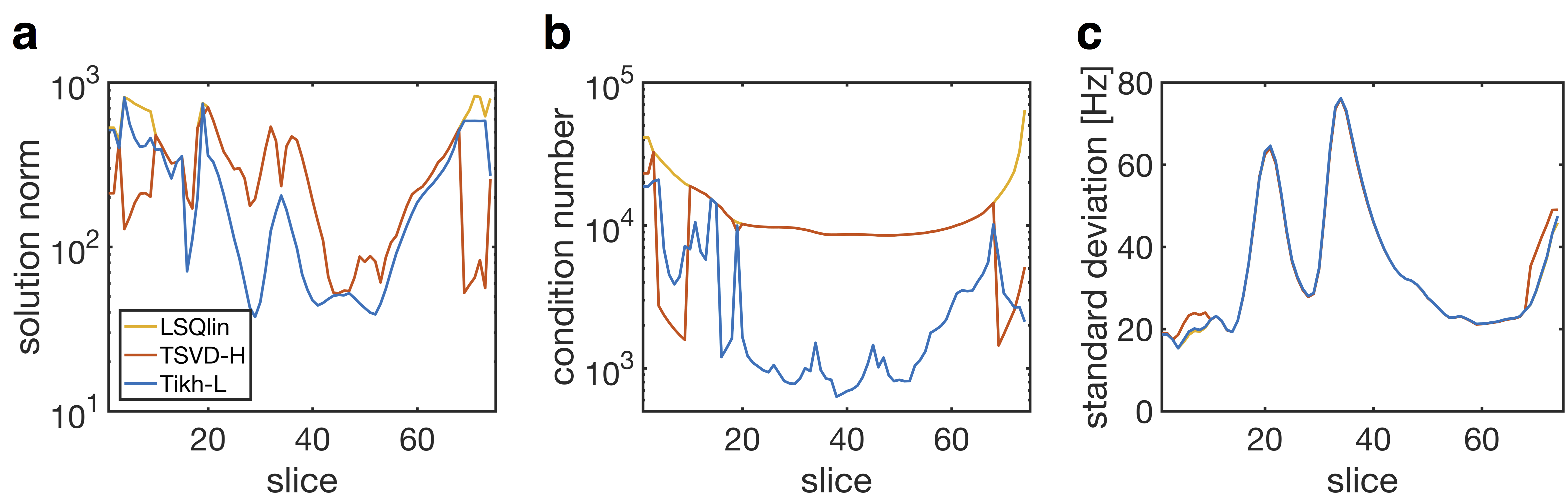
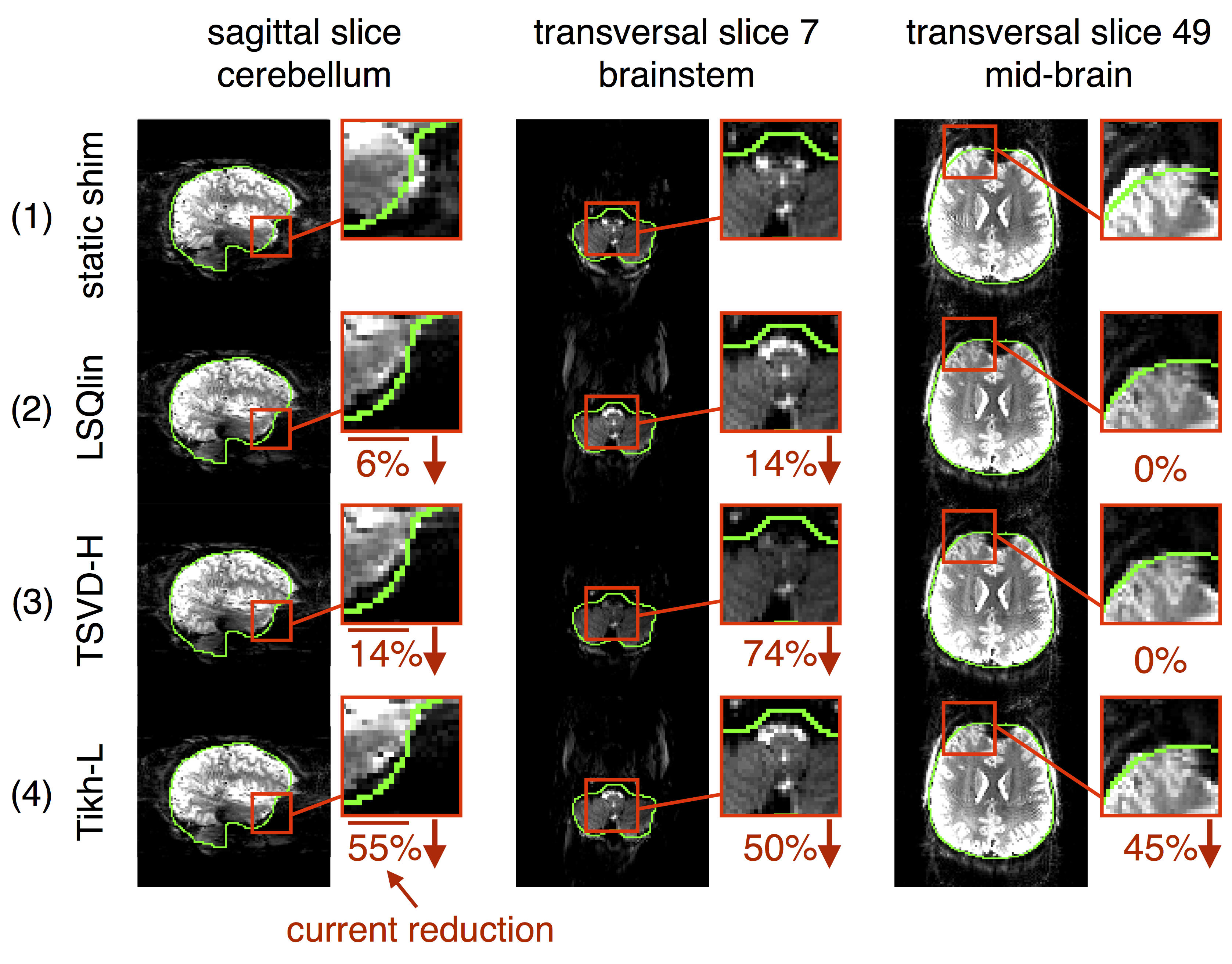
Fig. 4: EPI images acquired using the different shim calculation methods for dynamic shimming in one subject not included in the database. The columns from left to right contain a sagittal image through the temporal lobe, and transversal images at the brain stem and the mid-brain region. The rows from top to bottom show the EPI images acquired with the static shim (1), the dynamic shim with the LSQlin (2), TSVD-H (3) and Tikh-L (4) methods. The numbers located next to the images show the reduction in solution norm produced by the corresponding methods as compared to the unconstrained pseudoinverse.