Synopsis

Balanced Steady-State Free-Precession images are sensitive to T1, T2, off-resonance and Magnetization Transfer effects. Previously, Gloor et al extracted MT parameters from SSFP data, but required external T1 & B1 maps and did not account for off-resonance effects. Here we show that by incorporating the elliptical method of Shcherbakova et al, B0 can be measured and the need for an external T1 map removed. We present results covering the whole brain at 1.5mm isotropic voxel size acquired in 20 minutes. We also discuss an interesting asymmetry seen in the SSFP ellipse at low flip-angles.

Introduction

The balanced Steady-State Free Precession (bSSFP) sequence is strongly MT-weighted at short TRs and high flip-angles¹. Gloor et al² presented a method to calculate quantitative MT parameters from multiple bSSFP images, but only on-resonance and with an additional $$$T_1$$$ map. However, bSSFP suffers from off-resonance banding artefacts which limits the applicability of this method at high field.

Shcherbakova et al³ showed how to calculate $$$T_1\&T_2$$$ from bSSFP data using an elliptical signal model⁴, but disregarded MT effects. By combining these two methods we show that qMT parameters can be extracted from bSSFP data in a way that is robust to off-resonance artefacts at 3T in a clinically feasible scan-time.

Methods

We derived the bSSFP signal equation including off-resonance and exchange between free (subscript $$$f$$$) and restricted (subscript $$$r$$$) pools. Following², we first define:

$$A = 1 + F - E_{1r} f_{w}(F + f_{k})$$

$$B = 1 + f_{k} (F - E_{1r} f_{w} (F + 1))$$

$$C = F (1 - E_{1r}) (1 - f_{k})$$

$$f_{k} = e^{-(k_{f} + k_{r})TR}$$

where $$$F$$$ is the macromolecular proton fraction and $$$T_1$$$, $$$T_2$$$ & $$$k$$$ are the longitudinal relaxation, transverse relaxation and exchange rate of each pool. $$$f_{w}$$$ describes the rate of absorption of the restricted pool, with a lineshape approximated as a Gaussian with $$$T_{2r}=12 µs$$$². The resulting signal equations in elliptical form⁴ is then:

$$M = \frac{G (1 - a e^{- i \theta})}{1 - b\cos{\theta}}$$

where $$$M$$$ is the complex transverse magnetization, and

$$G = \frac{M_{0} (B (1 - E_{1f}) + C) \sin{\alpha}}{A - B E_{1f} \cos{\alpha} - E_{2f}^{2} (B E_{1f} - A \cos{\alpha})}$$

$$a = E_{2f}$$

$$b = \frac{E_{2f} (A - B E_{1f}) (\cos{\alpha} + 1)}{A - B E_{1f} \cos{\alpha} - E_{2f}^{2} (B E_{1f} - A \cos{\alpha})}$$

$$$\alpha$$$ is the flip-angle, $$$\theta=2\pi\Delta f_0 + \phi$$$ is the accrued phase due to off-resonance $$$\Delta f_0$$$ and phase increment $$$\phi$$$, and $$$M_0$$$ is the equilibrium magnetization. Figure 1 shows how the incorporation of MT changes the shape of the SSFP ellipse. $$$a$$$ is not affected by MT.

Monte Carlo simulations were conducted to investigate potential acquisition protocols. Calculating the MT parameters proceeded in two steps. First, for each simulated ellipse $$$G$$$, $$$a$$$ & $$$b$$$ were found using non-linear least squares. $$$T_{2f}$$$ was calculated from $$$a$$$. Then the remaining MT parameters were fitted to the values of $$$G$$$ and $$$b$$$. The chosen protocol consisted of four ellipses: two flip-angles (15° & 30°), each with two pulse-widths (256 and 1024 µs, one-lobed sinc) and TRs of 4.6 and 5.3ms respectively. Each ellipse had six phase-increments (0, 60, 120, 180, 240, 300°).

This protocol was implemented on a 3T GE MR750 scanner equipped with a 12-channel head coil. Scan time for the bSSFP images was 19 minutes (NEX=0.5, cylindrical k-space acquisition). The pulse profiles were simulated and multiplied by a Bloch-Siegert map⁵ to correct $$$B_1$$$ inhomogeneity. A healthy control was scanned, and the parameter maps found using the above fitting process. Regions-of-Interest were drawn in white and grey matter.

Results & Discussion

Figure 2 shows the Monte Carlo histograms. The Coefficient-of-Variation of each parameter was $$$M_0=2\%,F=11\%,k_f=23\%,T_{1f}=5\%,T_{2f}=4\%$$$. The high CoV of $$$k_f$$$ is due to a skewed distribution with many high values, but this did not affect fitting the other parameters.

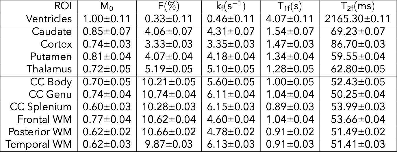
Figure 3 shows the acquired ellipse parameters for the 15° 1024µs data. The fitted residual is high in some white matter tracts, suggesting that a single ellipse cannot adequately describe the SSFP signal there. This is consistent with⁶, where the bSSFP signal was shown to be asymmetric in white matter. The residual is also high in blood vessels. Figure 4 shows the results of fitting the MT parameters to the ellipse parameters. ROI values are summarised in Table 1. The values of F are approximately 2/3rds of those in², but other parameters are broadly in line with literature values. The residual map does not exhibit the same structure as the ellipse residual in Figure 3.

Conclusions

Acknowledgements

References

1 - Bieri, O., & Scheffler, K. (2007). Optimized balanced steady-state free precession magnetization transfer imaging. Magnetic Resonance in Medicine, 58(3), 511–518. https://doi.org/10.1002/mrm.21326

2 - Gloor, M., Scheffler, K., & Bieri, O. (2008). Quantitative magnetization transfer imaging using balanced SSFP. Magnetic Resonance in Medicine, 60(3), 691–700. https://doi.org/10.1002/mrm.21705

3 - Shcherbakova, Y., van den Berg, C. A. T., Moonen, C. T. W., & Bartels, L. W. (n.d.). PLANET: An ellipse fitting approach for simultaneous T1 and T2 mapping using phase-cycled balanced steady-state free precession. Magnetic Resonance in Medicine, n/a--n/a. https://doi.org/10.1002/mrm.26717

4 - Xiang, Q.-S., & Hoff, M. N. (2014). Banding artifact removal for bSSFP imaging with an elliptical signal model. Magnetic Resonance in Medicine, 71(3), 927–933. https://doi.org/10.1002/mrm.25098

5 - Sacolick, L., & Wiesinger, F. (2010). B1 mapping by Bloch Siegert shift. Magnetic Resonance in Medicine. https://doi.org/10.1002/mrm.22357

6 - Miller, K. L., Smith, S. M., & Jezzard, P. (2010). Asymmetries of the balanced SSFP profile. Part II: White matter. Magnetic Resonance in Medicine, 63(2), 396–406.