0774
Deep neural network based framework for in-vivo axonal permeability estimation1Centre for Medical Image Computing and Dept of Computer Science, University College London, London, United Kingdom, 2CENIR, ICM, Paris, France, 3Inserm U 1127, CNRS UMR 7225, Sorbonne Universités, UPMC Univ Paris 06 UMR S 1127, Institut du Cerveau et de la Moelle épinière, ICM, Paris, France, 4INRIA, Université Côte d'Azur, Sophia-Antipolis, France, 5Parietal, CEA, INRIA, Saclay, Sophia-Antipolis, France, 6AP-HP, Hôpital Saint-Antoine, Paris, France, 7Hôpital de la Pitié Salpêtrière, Sorbonne Universités, UPMC Paris 06 UMR S 1127, Inserm UMR S 1127, CNRS UMR 7225, Institut du Cerveau et de la Moelle épinière, Paris, France, 8AP-HP, Hôpital de la Pitié Salpêtrière, Paris, France, 9Department of Brain Repair and Rehabilitation, Institute of Neurology, University College London, London, United Kingdom
Synopsis
This study introduces a novel framework for estimating permeability from diffusion-weighted MRI data using deep learning. Recent work introduced a random forest (RF) regressor model that outperforms approximate mathematical models (Kärger model). Motivated by recent developments in machine learning, we propose a deep neural network (NN) approach to estimate the permeability associated with the water residence time. We show in simulations and in in-vivo mouse brain data that the NN outperforms the RF method. We further show that the performance of either ML method is unaffected by the choice of training data, i.e. raw diffusion signals or signal-derived features yield the same results.
Introduction
This work investigates the potential of novel deep learning techniques for diffusion-weighted (DW) MRI microstructure imaging. We focus here on estimating the permeability of the axonal membrane, a potentially important biomarker for conditions affecting the myelin sheath1 such as Multiple Sclerosis. Recent work introduced for the first time a machine-learning (ML) approach2 based on a random Forest (RF) regressor to estimate the intra-axonal residence time τi (used as a measure of permeability) and showed that it outperforms approximate mathematical models (e.g. Kärger3).
Here we implement a novel ML framework based on deep neural networks (NN), which have been shown in other applications to outperform RF4. Furthermore, we investigate whether the raw DW-MRI signals (DW-signals) can provide better training than the signal-derived features (DW-features) used in Nedjati et al2.
Methods
We trained and tested the NN by constructing a mapping between DW-MRI data and ground truth microstructure parameters (intra-axonal volume fraction fi, intrinsic diffusivity d and τi ). We then compared it with the RF approach both in simulations and in in-vivo mouse brain data.
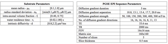
Synthetic Data: The training database is constructed from 11,000 synthetic DW-MRI signals simulated using Camino5, each corresponding to a unique substrate mimicking the in-vivo mouse data (Fig.1).
In-vivo Data: We use a healthy C57BL6J mouse scanned on a BrukerBioSpec 11.7T scanner using diffusion-weighted Pulsed-Gradients-Spin-Echo (DW-PGSE) sequence (protocol in Fig 1).
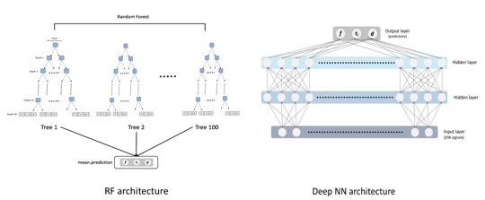
RF Regressor: We implemented an RF regressor with 100 trees and 20 maximum depth (Fig.2) using the scikit-learn Python toolkit6 and the default values for the other parameters. The regressor learns by implementing a greedy linear splitting process of the signal space guided by its associated tissue parameters provided as labels.
Deep NN: For this model (Fig.2) we use the open-source Keras7 library. The feed-forward NN is formed of an input layer that takes as an input the DW-signals/DW-features, two fully-connected hidden layers with 300 units and dropout and a final output layer for regression.
Training: We use separately DW-signals and DW-features for training and compare the performance of the two approaches for both RF and NN. The features, orientationally-invariant DTI parameters and spherical harmonics, were extracted as in Nedjati-Gilani et al2.
Results
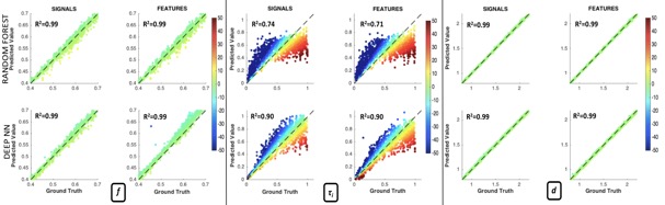
We observed very strong correlations between the predictions and the ground truth for all parameters on the noise free data (Fig.3). The NN outperforms the RF for both DW-signals and DW-features when predicting τi (RRF2=0.74/0.71 versus RNN2=0.90/0.90), providing a superior benchmark for the novel NN approach.
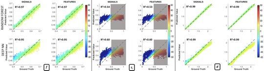
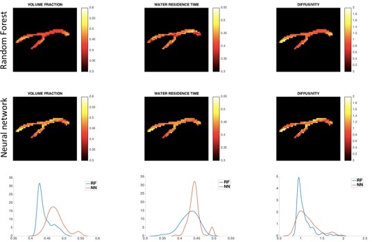
In the case of SNR=40, the NN continues to outperform the RF (Fig.4). All correlation coefficients are affected by noise; however, the parameters maintain a consistent, positive correlation. While the correlation coefficients for f and d remain high, that of τi drops to 0.60 for NN and 0.54 for RF, due to a loss of sensitivity caused by experimental noise. As the RF performs slightly better when fitted to DW-signals, we applied this approach to the manually segmented corpus callosum (CC) of the mouse brain (Fig 5).
The mouse CC parametric maps in Fig.5 show estimates within the physiologically plausible ranges for all three parameters. The in-vivo results are inherently difficult to validate, nevertheless, studies8,9 suggest values between 0.3s and 0.6s, consistent with our predictions. The mean predictions for τi and d across the CC are consistent between the RF and the NN. There is less variability in the NN estimations for τi, potentially attributable to the higher correlation coefficient seen in simulations. For f, the RF predictions are approximately 10% lower, an underestimation bias already observed by Nedjati et al2.
Discussion
The numerical simulations show that the NN framework outperforms RF. Although the presence of noise affects the performance of both approaches, NN continues to outperform RF also in realistic experimental conditions (SNR=40). Application to in-vivo data showed that both NN and RF provide histologically plausible parameters maps for mouse CC. NN predictions of τi have a narrower variability compared to RF which is potentially indicative of a higher robustness to noise of the NN approach. We additionally showed that the raw DW-signals are not performing better but are equally informative as the DW-features introduced by Nedjati et al2. Future work will optimise the NN architecture, improve sequences for sensitivity to permeability and conduct further validation.Conclusion
This work introduces a novel deep NN framework for the DW-MRI based estimation of permeability, representing a step forward in the construction of increasingly robust and reliable ML-based approaches for tissue microstructure estimation. The framework proposed here can be extended to other more complex biophysical models improving the estimation of microstructure parameters.Acknowledgements
This work was supported by EPSRC (EP/G007748, EP/I027084/01, EP/L022680/1, EP/M020533/1, N018702), EPSRC-funded UCL Centre for Doctoral Training in Medical Imaging (EP/L016478/1), Spinal Research, UK MS Society and NIHR Biomedical Research Centre at University College London Hospitals. The research leading to these results received funding from the programs 'Institut des neurosciences translationnelle' ANR-10- IAIHU-06 and 'Infrastructure d’avenir en Biologie Santé' ANR-11-INBS-0006.References
1. Nilsson, M. et al. The role of tissue microstructure and water exchange in biophysical modelling of diffusion in white matter. Magnetic Resonance Materials in Physics, Biology and Medicine 26.4:345-370, 2013.
2. Nedjati-Gilani, G., et al. Machine learning based compartment models with permeability for white matter microstructure imaging. NeuroImage 150:119-135, 2017.
3. Kärger,, J., Principles and applications of self-diffusion measurements by nuclear magnetic resonance. Adv Magn Reson 12:1-89, 1988.
4. Tanno, R. et al., Bayesian Image Quality Transfer with CNNs: Exploring Uncertainty in dMRI Super-Resolution. arXiv preprint arXiv:1705.00664 2017.
5. Cook, P. A., et al. Camino: Open-Source Diffusion-MRI Reconstruction and Processing, 14th Scientific Meeting of the International Society for Magnetic Resonance in Medicine, Seattle, WA, USA, p. 2759, 2006.
6. Pedregosa, F. Scikit-learn: Machine Learning in Python. JMLR 12, 2825-30, 2011.
7. Chollet, F. et al. Keras, GitHub (https://github.com/fchollet/keras), 2015.
8. Quirk, J. D., et al. Equilibrium water exchange between the intra‐and extracellular spaces of mammalian brain. Magnetic resonance in medicine 50.3:493-499, 2003.
9. Finkelstein, A., Water and nonelectrolyte permeability of lipid bilayer membranes. The Journal of general physiology 68.2:127-135, 1976.
Figures