0773
Progressively Distribution-based Rician Noise Removal for Magnetic Resonance Imaging1Department of Electronic Information Engineering, Nanchang University, nanchang, China, 2Lauterbur Research Centre for Biomedical Imaging, Shenzhen Key Laboratory for MRI, Shenzhen Institutes of Advanced Technology, Shenzhen, China
Synopsis
Different from the existing MRI denoising methods that utilizing the spatial neighbor information around the pixels or patches, this work turns to capture the pixel-level distribution information by means of supervised network learning. A wide and progressive network learning strategy is proposed, via fitting the distribution at pixel-level and feature-level with large convolutional filters. The whole network is trained in a two-stage fashion, consisting of the residual network in pixel domain with batch normalization layer and in feature domain without batch normalization layer. Experiments demonstrate its great potential with substantially improved SNR and preserved edges and structures.
Introduction:
Recent researches on magnitude MRI reconstruction focuses on the proper modeling of the resulting Rician noise contaminated data. It’s well recognized that Rician noise is signal-dependent and the denoising task is challenge, which is especially problematic in low SNR regimes. Different from the existing denoising methods utilizing the spatial neighbor information around the pixels or patches [1][2], this work turns to capture the pixel-level distribution information by means of supervised network learning. The main contributions include: 1) a wide and progressive network learning strategy is proposed, via fitting the distribution at pixel-level and feature-level with large convolutional filters; 2) Batch normalization (BN) operator is used in the first subnetwork, while no BN operator used in the second subnetwork.Theory:
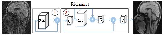
A flowchart of the proposed Riciannet is shown in Fig. 1. It learns the whole Rician noise distribution via two subnetworks. The first subnetwork is to employ the residual network (ResNet) to generate a good preliminary estimate by increasing the convolutional neural network (CNN)’s width with larger receptions and more channels. The second subnetwork employs ResNet in feature domain to further improve the restoration quality. The model is trained in a progressive fashion. i.e., it first trains the first subnetwork and then employs the intermediate trained net to partly initialize the whole network at the second training stage.
I. Noise Removal via Distribution Approximation:
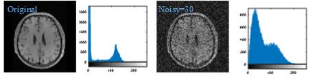
If both real and imaginary parts of a signal x are corrupted with uncorrelated Gaussian noise ( $$${n_1}$$$ and $$${n_2}$$$ ) with equal variance (0, $$${\sigma ^2}$$$ ), the envelope of the magnitude signal $$$y = \sqrt {{{\left( {x + {n_1}} \right)}^2} + n_2^2}$$$will follow a Rician distribution [1]. It can be observed in Fig. 2 that as the noise level in $$$x$$$ increases, the distribution of $$$y$$$ will close to Rician distribution. We tend to learn this distribution via integrating the Gaussian distribution in pixel domain and sparse distribution in feature domain.
II. Wide and Progressive Network:
Although CNN based models have achieved great success, the long-term dependency problem is rarely realized as the network depth grows. Recent works [3][4][5] revealed that, with exploration of the “width” of the network, the performance will largely improve. The number of neurons and weights in the convolution (Conv) layer are referred to as the width of a CNN, i.e., the number of layers L, the number of filters K and the size of filters F . In this work, besides of increasing the CNN’s width with larger receptions and more channels, we enhance the model width via using residual block in feature domain, as shown in Fig. 1. Furthermore, the model is trained in a progressive fashion. i.e., we first train the first subnetwork and then employ the intermediate net to partly initialize the whole network at the second training stage.
III. (No) Batch Normalization:
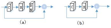
One key to the success of many state-of-the-art network is to use the BN [3][4][6] (Fig. 3). They stated that BN reduces the scale and initialization sensitivity and alleviates to get stuck via normalizing the weights. On the other hand, a few works revealed that the network’s performance can be improved by removing BN layers [5], as BN layers may get rid of range flexibility from networks. Therefore, we adopt a progressive and distribution fitting network procedure to benefit from the strengths of both. First, from the viewpoint of distribution fitting, BN operator is utilized in the first subnetwork for approaching Gaussian distribution, while avoiding BN operator in the second subnetwork for approximating sparse distribution. The series structure is prone to approach the general non-Gaussian distribution. Second, from the viewpoint of non-linearity optimization, the first subnetwork is intermediately trained and employed to partly initialize the whole network at the second training stage. Therefore, the whole network can be easily trained.Materials and Methods:
We use the Brainweb dataset containing T1,T2 and PD images as training set. The patch size is 41×41. In each Residual block, L=5, K=128 and F=7×7. Besides, in the second subnetwork, the filter size used in feature generation that dubbed as “C” in Fig. 1 is 64. The model is trained with ADAM optimizer and implemented with Caffe framework using NVIDIA Titan X GPUs.Results:
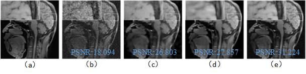
Fig. 4 compares three images restored using UNLM [1] in (c), BM3D-NIDe-VST [2] in (d), and the proposed RicianNet algorithm in (e). Obviously, the denoising result of RicianNet provides much visual improvement and exhibits less blurring artifacts. The PSNR value of RicianNet outperforms UNLM with gains over 4.42dB and BM3D-NIDe-VST with improvement of 3.37dB.Conclusion:
In this work, we demonstrated that the wide and progressive network, via fitting the distribution at pixel-level and feature-level with large convolutional filters, can successfully be applied to Rician denoising. Compared with the conventional de-noising methods, it substantially improves SNR and preserves edges and structures.Acknowledgements
the National Natural Science Foundation of China under 61661031, 61362001, 61365013.References
[1] Manjón J V, et al. MIA, 2008, 12(4):514. [2] Elahi P. et al ICASSP, 2014; 6612-6616. [3] Woong Bae, et al. 2017 arXiv:1161.06345. [4] Liu Peng, Ruogu Fang, 2017 arXiv: 1707.05414v3. [5] Lim B, et al. CVPRW. IEEE, 2017:1132-1140. [6] Zhang K, et al. IEEE TIP, 2017, 26(7):3142-3155.Figures