0716
A Patch-Based Convolutional Neural Network Model for the Diagnosis of Prostate Cancer using Multi-Parametric Magnetic Resonance Images1Shanghai Key Laboratory of Magnetic Resonance, East China Normal University, Shanghai, China, 2Department of Radiology, the First Affiliated Hospital with Nanjing Medical University, Nanjing, China, 3MR Scientific Marketing, Siemens Healthcare, Shanghai, China
Synopsis
We proposed a patch-based convolutional neural network (CNN) model to distinguish prostate cancer using multi-parametric magnetic resonance images (mp-MRI). Our CNN model was trained in 182 patients including 193 cancerous (CA) vs. 259 normal (NC) regions, and tested independently in 21 patients including 21 CA vs 31 NC regions. The model produced an area under the receiver operating characteristic curve of 0.869, sensitivity of 90.5% and specificity of 67.7% for the differentiation of CA from normal regions, showing its potential for the diagnosis of prostate cancer in clinical application.
Introduction
Prostate cancer (CA) is the most common malignancy and second leading cause for death for men of western countries. Multi-parametric MRI (mp-MRI) has been recognized a reliable tool for detecting, staging and classifying CA. Recently, growing evidences indicate that machine learning methods could be a potential alternative to conventional methodologies with respects to diagnostic effectiveness in medical imaging.1 However, these algorithms require pre-processing of large numbers of input features before data modeling, the variability is thus not avoidable. Convolutional Neural Network (CNN) has achieved great success in classification, detection, and reconstruction of the medical images.2 One advantage of CNN is that it can automatically find useful features from mp-MR images. Here we proposed a patch-based CNN model to distinguish CA from normal tissue using mp-MRI.Methods
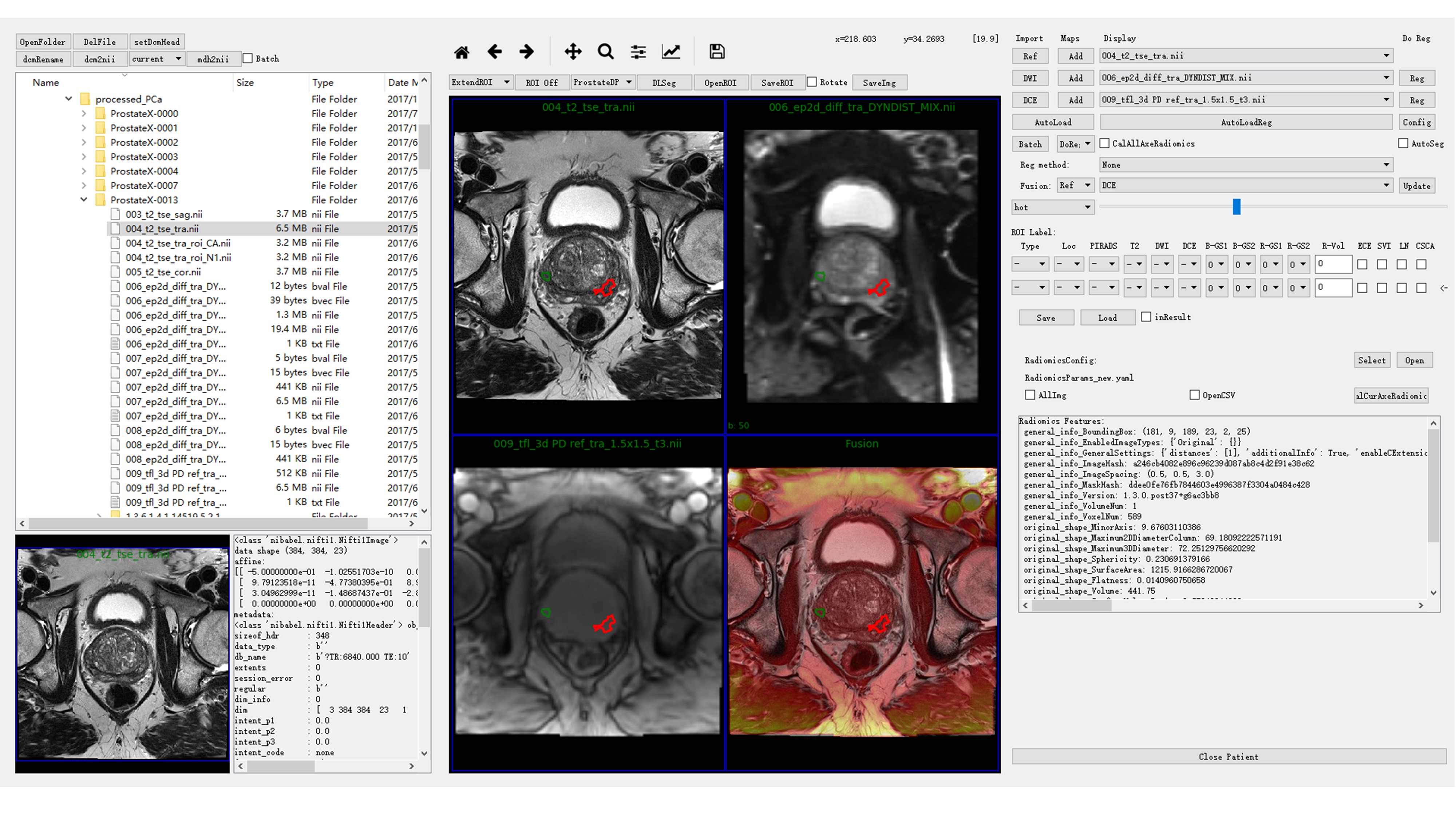
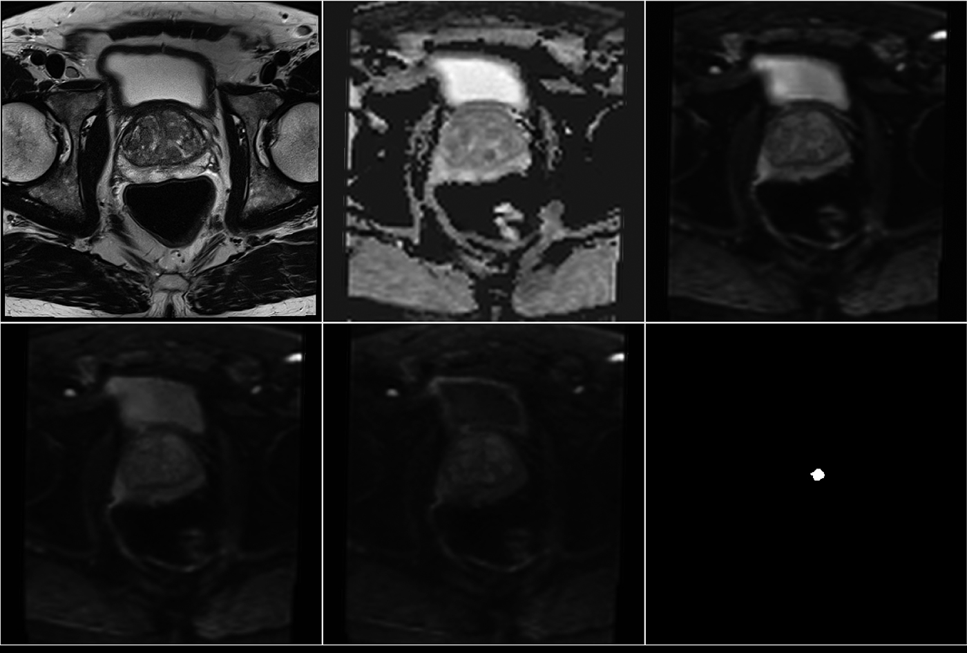
We utilized the 182 mp-MRI data downloaded from PROSTATEx to train our CNN model.3 A few preprocessing steps were done with our in-house software written in Python (DeepOncoAnalysis, Figure 1). Firstly, the diffusion weighted (DW) images of different b values were spatially aligned for apparent diffusion coefficient (ADC) calculation using Elastix.4 Then, the DW and ADC images were aligned to T2W image for voxel-wised analysis. One radiologist drew the candidate region-of-interest (ROI) on T2W image and labeled CA or NC regions based on histologic-radiologic correlation of prostate provided by PROSTATEx (Figure 2). We used 2D patches (65 x 65) centered at the center of the labeled ROI for all modalities in order to train the CNN model.
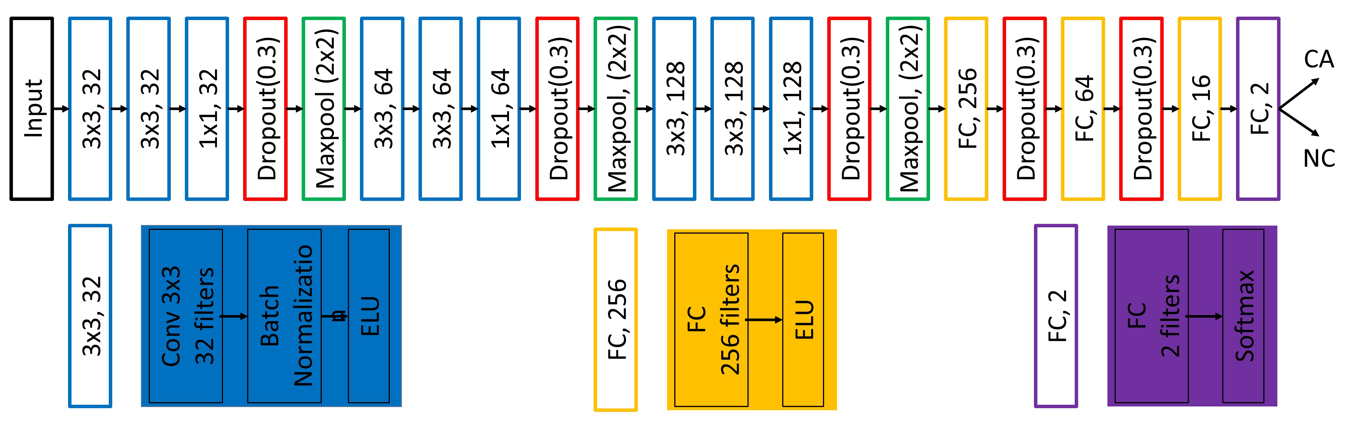
We designed a patch-based CNN model (Figure 3) with multi-modality inputs (transverse T2W, DWI with b value 50, 400 and 800 s/mm2, and the corresponding ADC map) and binary outputs of CA / non-cancer (NC) to classify the candidate region. For robust model training, we utilized a few tricks: a) Batch-normalization and dropout to overcome the over-fitting problem; b) 1 x 1 layer before max-pooling to increase the depth of the network for capturing more abstract features; 3) Exponential Linear Unit (ELU) guarantee weights update even when convolutional results are negative. The training dataset came from 182 patients including 452 candidate regions (CA / NC = 193 / 259) for our CNN model. Another 21 patients including 52 candidate regions (CA / NC = 21 / 31) was chosen for testing our CNN model. After that CNN model gives the probability of the candidate region belonging to CA, another hyper-parameter was chosen to apply threshold for the classification. The area under the receiver operating characteristic (ROC) curve (AUC) was calculated to evaluate the model. Our CNN model was built with Keras on TensorFlow, and run on NVIDIA Titan X for 12 hours on training.
Results
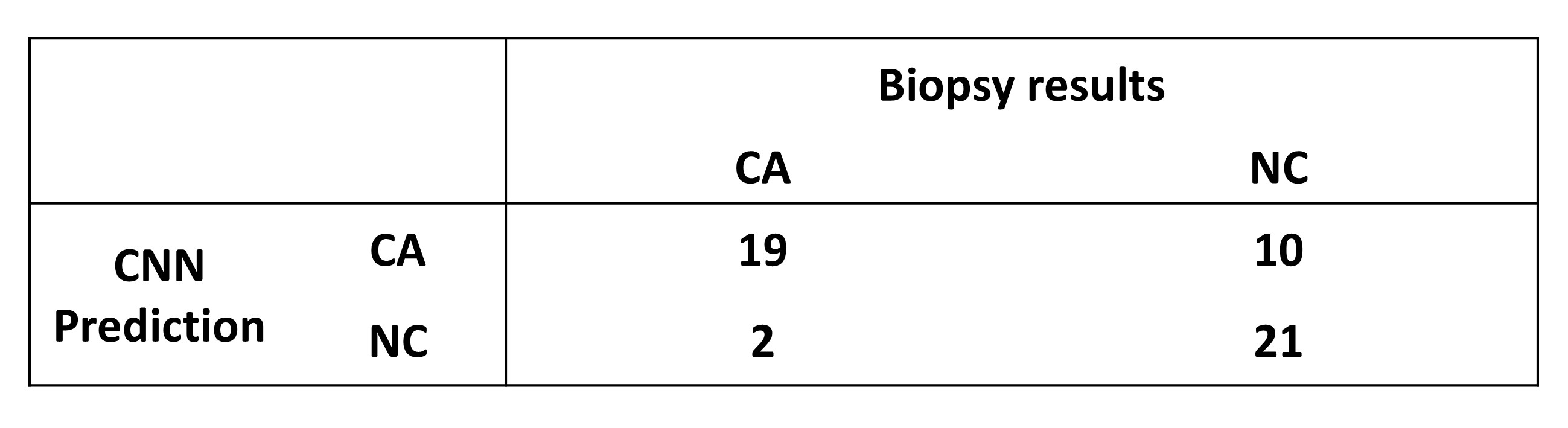
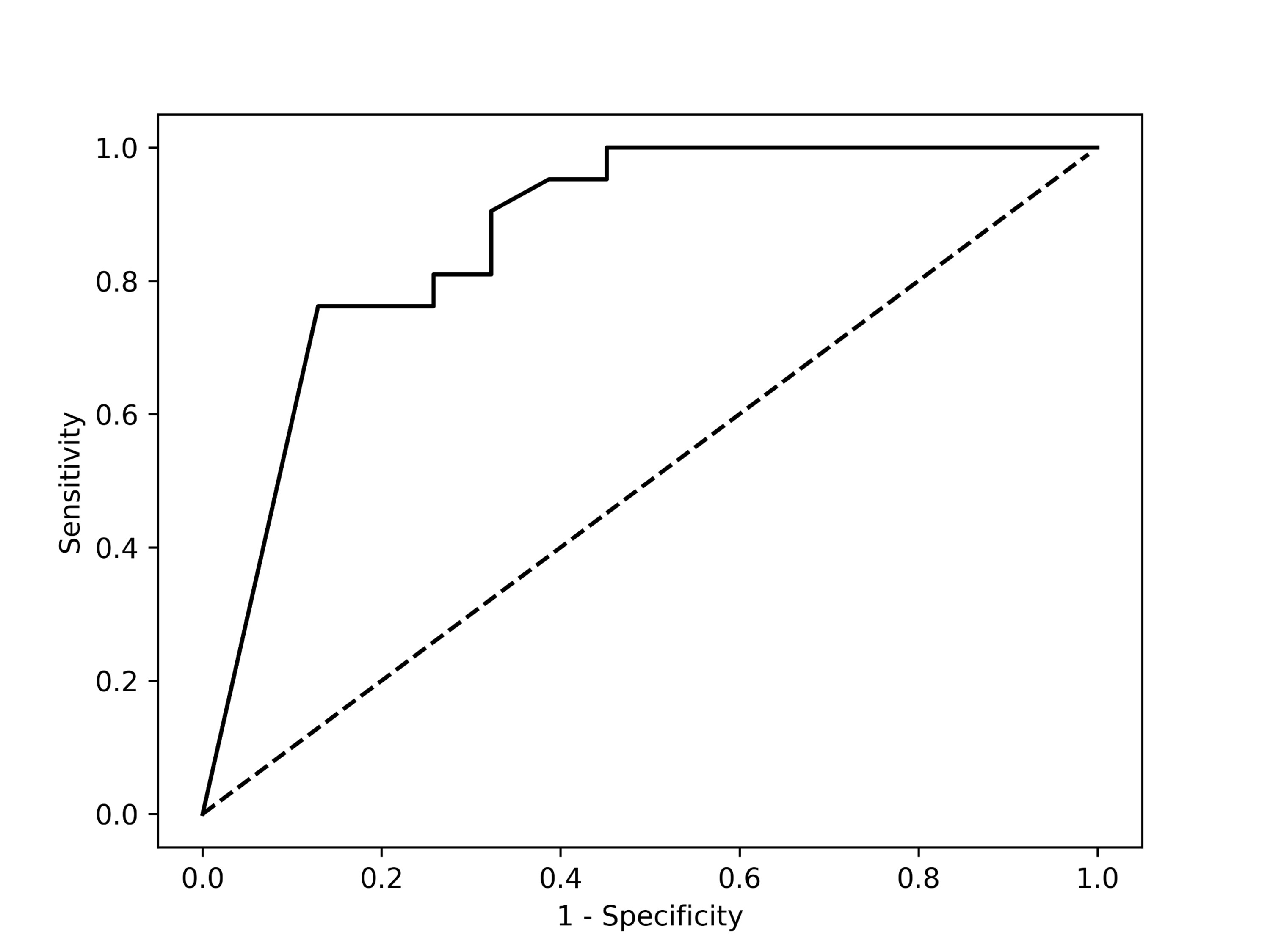
Figure 4 showed the statistical results for the testing data by the trained CNN model with threshold value equaling to 0.5. Our CNN model could give sensitivity / specificity of 90.5% / 67.7% on the CA from mp-MR images and give 0.869 AUC for the testing data (Figure 5). When the sensitivity was close to 100%, we had to suffer about specificity of 50%, which costed much to classify the false-positive candidate region. When the specificity was about 90%, sensitivity of roughly 75% might make radiologists worried of missing CA. For the training data, our CNN model estimated AUC very close to 1.0.Discussion and Conclusion
CNN showed its potential for CA classification in clinical diagnosis. Compared with other algorithms based on machine learning, CNN works without any features designed manually. CNN has high sensitivity to detect the CA but also yields some false-positive candidate region. A possible reason is that CNN is hard to classify the CA in transitional zone and central zone due to the complex tissue structures therein, and overfitting is more likely to occur. Data augmentation and more mp-MR images with biopsy results may help solve this problem. Furthermore, the addition of more modalities, such as DCE images and Ktrans map, or the use of 3D structure information may increase the specificity and AUC of CNN.Acknowledgements
The study was supported by the key project of the National Natural Science Foundation of China (61731009).References
- Chung A, Shafiee M, Kumar D, et al. Discovery Radiomics for Multi-Parametric MRI Prostate Cancer Detection. arXiv preprint arXiv:1509.00111, 2015.
- Litjens G, Kooi T, Bejnordi B, et al. A survey on deep learning in medical image analysis. arXiv preprint arXiv:1702.05747, 2017.
- Litjens G, Debats O, Barentsz J, et al. Computer-aided detection of prostate cancer in MRI, IEEE Transactions on Medical Imaging 2014;33:1083-1092.
- Klein S, Staring M, Murphy K, et al, elastix: a toolbox for intensity based medical image registration, IEEE Transactions on Medical Imaging, 2010; 29(1): 196-205.
Figures