Synopsis

MR fingerprinting provides quantitative parameter maps from a single acquisition, but it also has the potential to reduce exam times by replacing traditional protocol sequences with synthetic contrast-weighted images. We present an empirical "artifact noise" model that makes it possible to train neural networks that successfully transform noisy and aliased MRF signals into parameter maps, which are then used to synthesize contrast-weighted images. We also demonstrate that a trained neural network can directly synthesize contrast-weighted images, bypassing incomplete simulation models and their associated artifacts.

Introduction

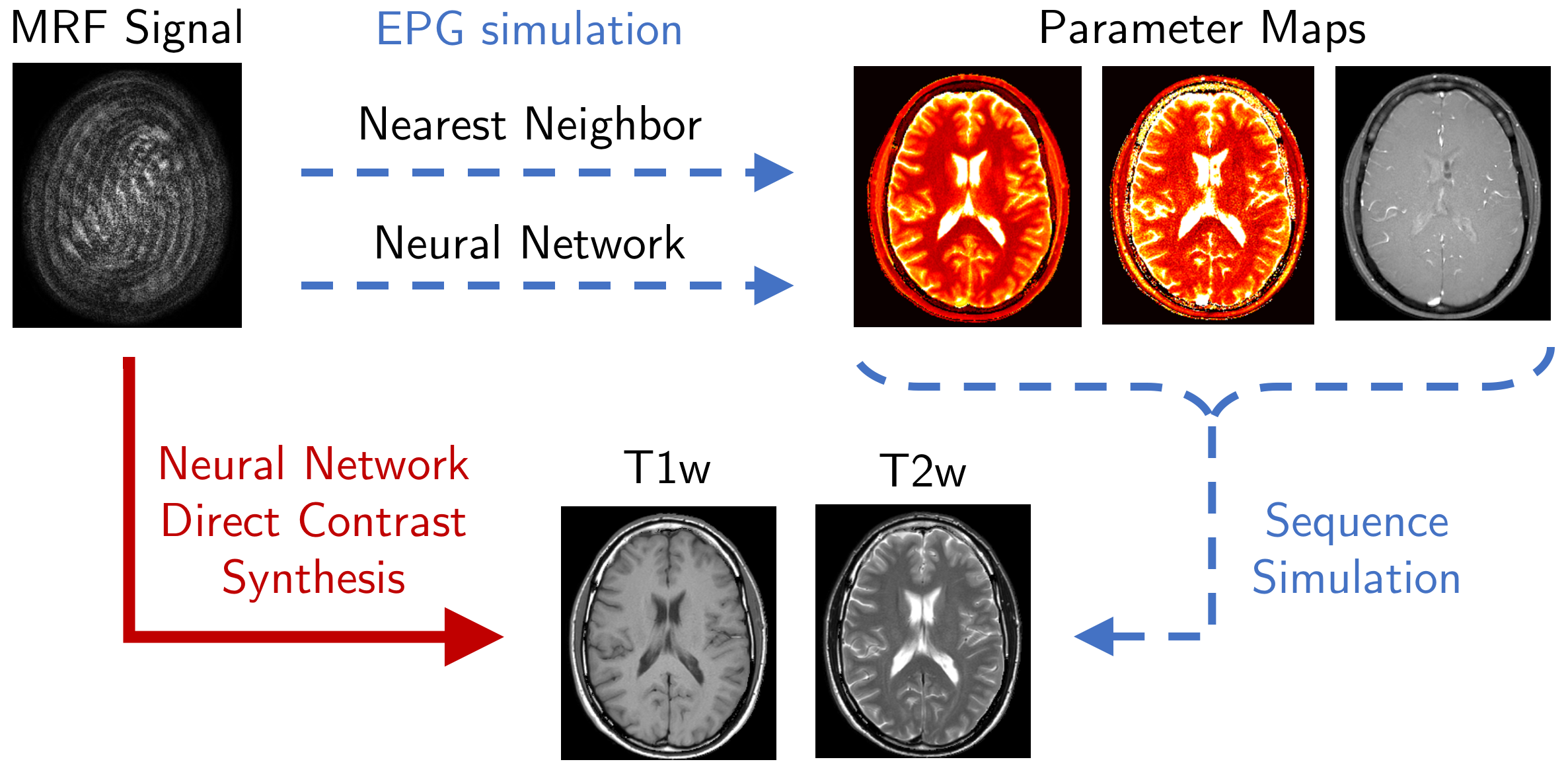
Magnetic resonance fingerprinting (MRF) can generate quantitative maps of tissue and system parameters (PD,T1,T2,B0,B1) from a single acquisition¹. MRF also has the potential to replace standard radiological sequences by using the parameter maps to indirectly synthesize contrast-weighted images, such as T1- and T2-weighted images, (Figure 1, dotted-blue lines).

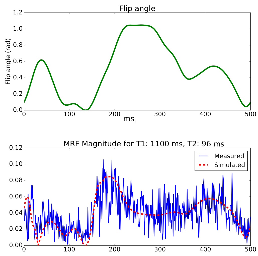
Previous work has demonstrated that neural networks can be an effective and efficient means generate parameter maps from MRF^2,3. These methods add Gaussian noise to simulated MRF data to train neural networks that are robust to acquisition noise. As MRF signals are highly under-sampled, Gaussian noise does not adequately model the severe incoherent aliasing artifacts, which are signal dependent and difficult to simulate (Figure 2).

In order to train neural networks to generate parameter maps despite noise coupled with aliasing, we propose using an empirical “artifact noise” model. The basic idea is to obtain samples of “artifact noise” from MRF acquisitions. By subtracting measured MRF signals from their nearest simulated signal, we obtain samples which contain mostly “noise artifacts” and can be used to augment the neural network training set.

The concept of MRI synthesis dates back to 1985⁴, and techniques such as QRAPMASTER/MAGiC⁵ have recently been shown to produce clinically viable images⁶. MRF contains rich parametric information and can be used for contrast synthesis. However, MRI synthesis from parameters is significantly limited by biases due to effects that are difficult to simulate, e.g. time varying signals, partial voluming, flow, diffusion, and magnetization transfer.

We propose training neural networks to directly synthesize contrast-weighted images from MRF data, bypassing insufficient parameter modeling (Figure 1, solid-red line). Direct synthesis networks must be trained with contrast-weighted images registered to acquired MRF data, but ground truth contrast-weighted images are part of routine examinations and can be much easier to acquire than lengthy ground truth parameter mapping sequences.

Methods

in-vivo dataset

We scanned 12 volunteers with a 1.5T Philips Ingenia scanner using 13 receive channels. We acquired three consecutive axial head sequences: SE T1-weighted (TE=15,TR=450), TSE T2-weighted (TE=110,TR=2212), and a bFFE MRF sequence with 500 repetitions, constant (TE=3.3,TR=20), and flip angles shown in Figure 2. The spiral MRF acquisition was reconstructed with gridding and Philips CLEAR. We used the data from eight volunteers for training, two for validation, and two only for final test results.

Empirical "artifact noise" model

Our empirical noise model considers three factors: noise signature, SNR, and phase.

1) Artifact noise signature: Given a measured MRF signal, $$$y$$$, and its nearest simulated signal, $$$x$$$, we compute a sample of "artifact noise":$$noise=y-\alpha x$$where $$$\alpha$$$ is the signal scaling factor computed from $$$\text{argmin}_\alpha||y-\alpha x||_2$$$.

2) SNR: Proton density affects signal strength at each pixel, independent from T1, T2, and acquisition noise. For this reason, we collect samples of estimated SNR:$$SNR=\frac{||\alpha x||_2}{||noise||_2}$$

3) Phase: Because the absolute phase of measured signal is arbitrary, we also include a random phase shift to both our simulated signal and our sampled noise.

We combine these three factors to create a noisy version for each simulated training signal $$$x$$$:$$x_{noisy}=x\cdot e^{j\phi_1}+\frac{1}{SNR_i}\frac{noise_k}{||noise_k||_2}e^{j\phi_2}$$where $$$i$$$ and $$$k$$$ are random indices and $$$\phi_1$$$ and $$$\phi_2$$$ are random angles.

Indirect contrast synthesis

We simulated MRF signals with the extended phase graph (EPG) algorithm^7,8, and used cosine similarity to match nearest neighbors as in Ma et al¹.

Our neural networks for parameter mapping uses the 2-channel real/imaginary architecture from Virtue et al² without batch normalization. The networks were trained with 100,000 simulated signals augmented with our empirical artifact noise model and compared to networks trained using a Gaussian noise model with pSNR values 2.5, 5, and 10.

The nearest neighbor and neural network parameter maps were converted to T1-weighted and T2-weighted images by simulating spin echo sequences:$$SE=PD\cdot e^{-TE/T2}(1-e^{-(TR-TE)/T1})$$

Direct contrast synthesis

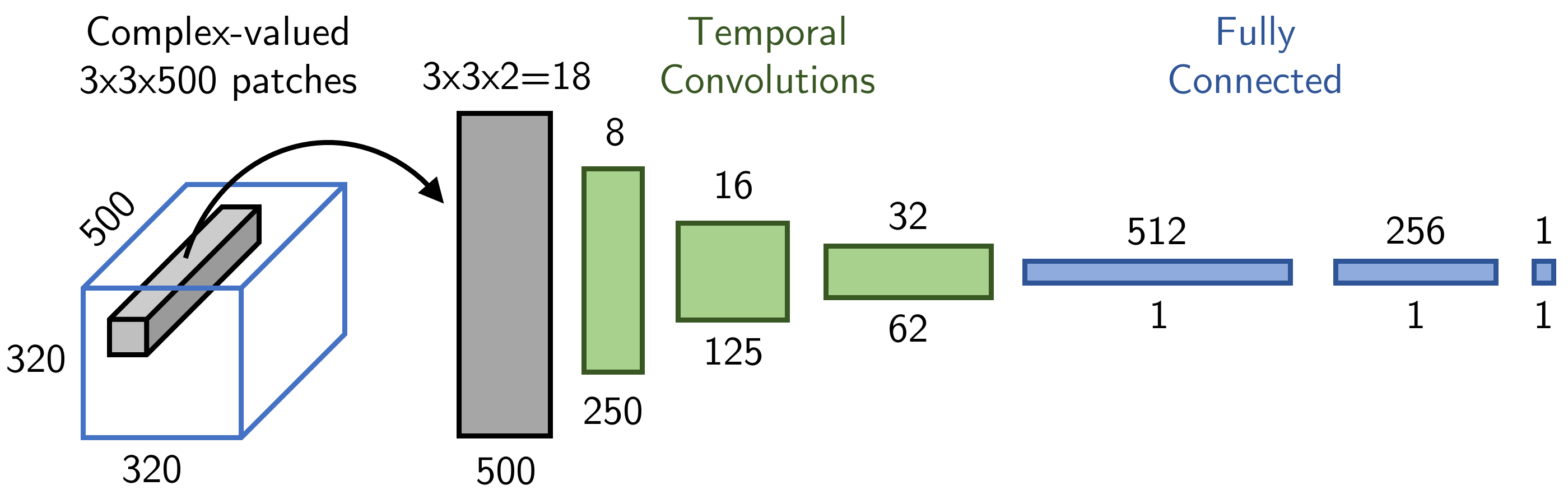
The neural network for direct contrast synthesis was trained on 3.7 million 3x3 patches from the in-vivo MRF data with no augmentation, (Figure 3).

Results

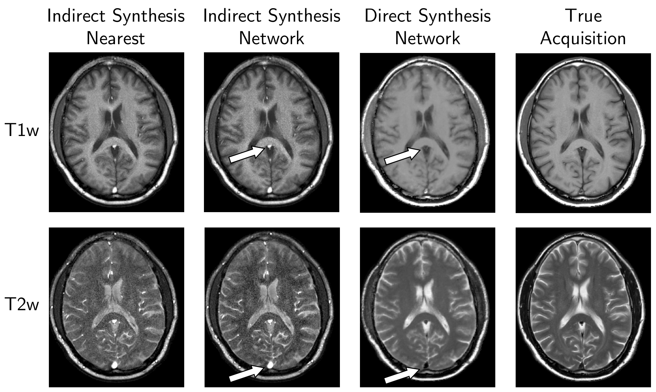
Direct contrast synthesis consistently produced higher quality results than either of the indirect contrast methods, both of which contain significant artifacts, especially in the vasculature and CSF (Figure 4).

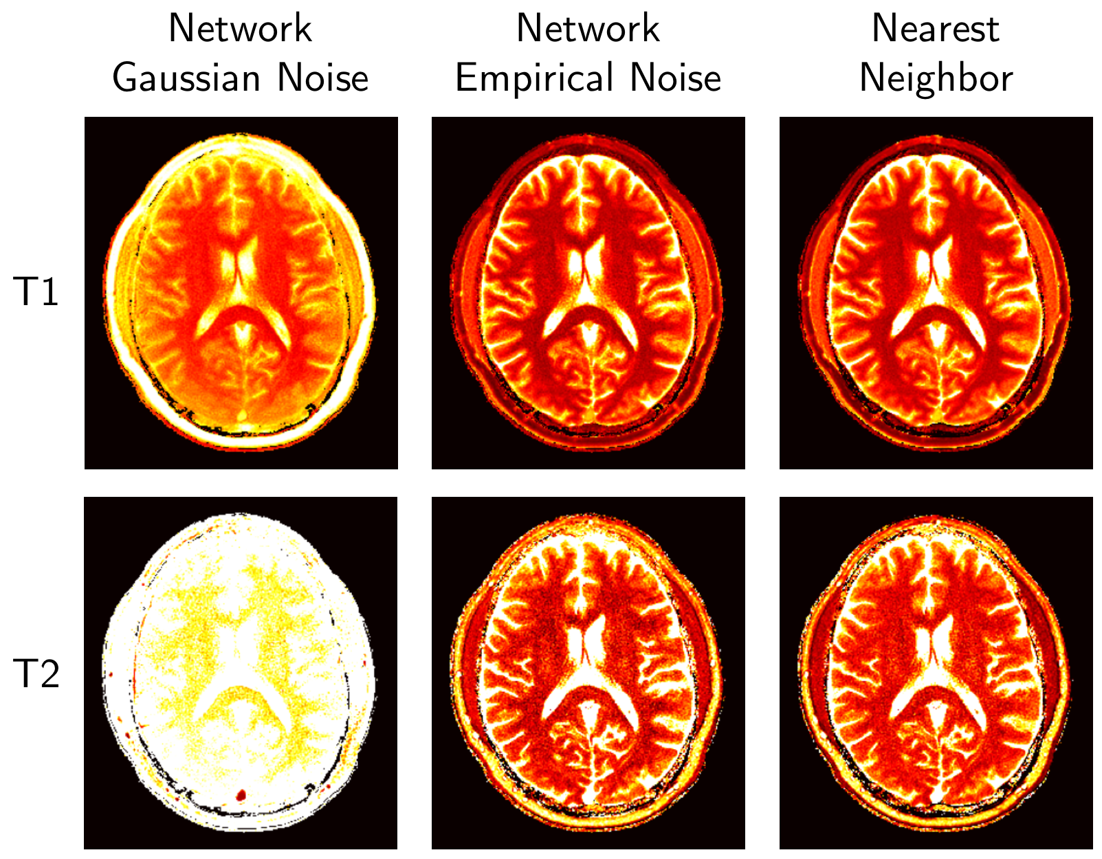
Figure 5 shows that the network trained with our empirical artifact noise performs as well as nearest neighbor, whereas the network with Gaussian noise fails to produce viable parameter maps.

Discussion and Conclusion

We demonstrate that our empirical noise model significantly outperforms standard Gaussian noise models when training a neural network to produce parameter maps from in-vivo MRF acquisitions.

We show that our deep learning model for direct contrast synthesis can bypass incomplete simulation models and their associated artifacts.

We look forward to training with a larger dataset and applying our synthesis methods to additional contrast sequences, such as FLAIR.

Acknowledgements

References

1. D. Ma, V. Gulani, N. Seiberlich, K. Liu, J. L. Sunshine, J. L. Duerk, and M. A. Griswold, “Magnetic Resonance Fingerprinting,” Nature, vol. 495, no. 7440, pp. 187–192, 2013.

2. P. Virtue, S. X. Yu, and M. Lustig, “Better than Real: Complex-valued Neural Networks for MRI Fingerprinting,” in Proceedings of IEEE International Conference on Image Processing, 2017.

3. O. Cohen, B. Zhu, and M. Rosen, “Deep Learning for Fast MR Fingerprinting Reconstruction,” in Scientific Meeting Proceedings of International Society for Magnetic Resonance in Medicine, 2017, p. 688.

4. S. A. Bobman, S. J. Riederer, J. N. Lee, S. A. Suddarth, H. Z. Wang, B. P. Drayer, and J. R. MacFall, “Cerebral Magnetic Resonance Image Synthesis,” American Journal of Neuroradiology, vol. 6, no. 2, pp. 265–269, 1985.

5. J. B. M. Warntjes, O. D. Leinhard, J. West, and P. Lundberg, “Rapid Magnetic Resonance Quantification on the Brain: Optimization for Clinical Usage,” Magnetic Resonance in Medicine, vol. 60, no. 2, pp. 320–329, 2008.

6. L. N. Tanenbaum, A. J. Tsiouris, A. N. Johnson, T. P. Naidich, M. C. DeLano, E. R. Melhem, P. Quarterman, S. X. Parameswaran, A. Shankaranarayanan, M. Goyen, and A. S. Field, “Synthetic MRI for Clinical Neuroimaging: Results of the Magnetic Resonance Image Compilation (MAGiC) Prospective, Multicenter, Multireader Trial,” American Journal of Neuroradiology, 2017.

7. J. Hennig, “Multiecho Imaging Sequences with Low Refocusing Flip Angles,” Journal of Magnetic Resonance (1969), vol. 78, no. 3, pp. 397–407, 1988.

8. M. Weigel, “Extended Phase Graphs: Dephasing, RF Pulses, and Echoes - Pure and Simple,” Journal of Magnetic Resonance Imaging, vol. 41, no. 2, pp. 266–295, 2015.