0658

Simultaneous Relaxometry and Segmentation of Human Brain through a Deep Neural Network

Peng Cao¹, Jing Liu¹, Shuyu Tang¹, Andrew Leynes¹, and Peder Larson¹

¹Department of Radiology and Biomedical Imaging, University of California at San Francisco, San Francisco, CA, United States

Synopsis

This study demonstrated a method for 3D simultaneous relaxometry and segmentation of human brain tissues through a deep neural network. Ranges of T1 and T2 values for gray matter, white matter and cerebrospinal fluid (CSF) were used as the prior knowledge. The proposed method can directly generate brain T1 and T2 maps in conjunction with segmentation of gray matter, white matter and CSF, and in particular was robust for relaxometry/segmentation in the challenging region of deep brain nuclei.

Purpose

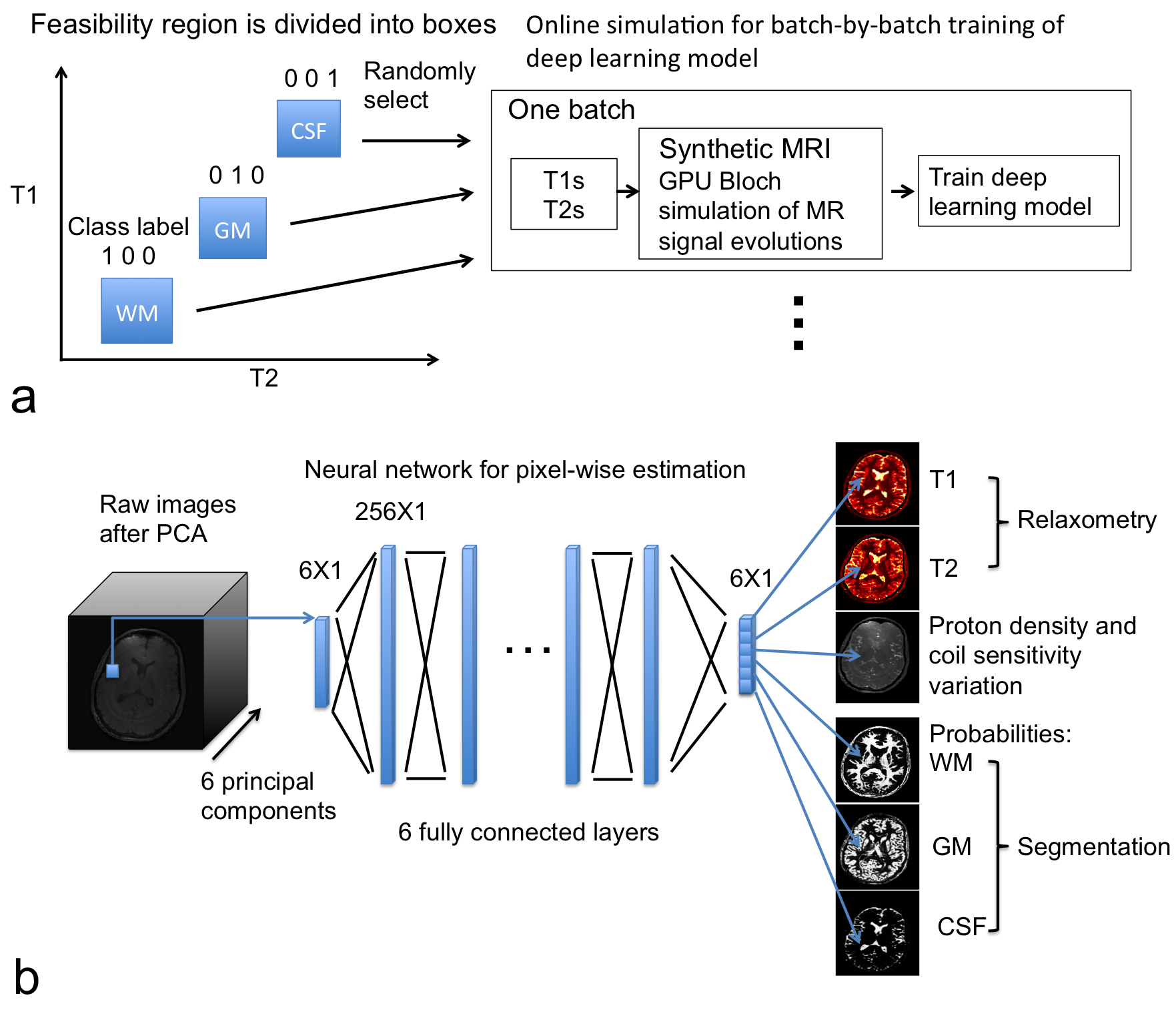
Quantitative MRI allows direct measurement of biophysical parameters of normal and pathological tissues in vivo ^1–4 with applications in tissue segmentation/classification ^5–7 and macromolecule quantification ^8–11. A promising method for quantitative MRI is MR fingerprinting (MRF), which uses a dictionary to solve the Bloch equation for deriving T1 and T2 values ¹², and T1 and T2 values are assumed to align with grid entries in the parameter space ¹². Meanwhile, T1 and T2 values in biological tissues are often positively associated with each other, e.g. the T1 and T2 values of gray matter are both longer than those of white matter ^13,14. We trained a neural network for quantitative MRI measurements to “understand” this association (e.g. a simple box constraints as shown in Fig. 1a) with given ranges of T1 and T2 values for gray matter (GM), white matter (WM) and cerebrospinal fluid (CSF). Our results showed that the deep neural network could directly generate 3D T1 and T2 maps in conjunction with the segmentation of gray matter, white matter and CSF for in vivo human brain imaging.

Methods

MRI sequence and in vivo data acquisition: An inversion-prepared balanced steady state free precession (bSSFP) sequence was used for acquiring the in vivo dynamic brain images ^15,16. Parameters included constant flip angle = 30°, constant TR/TE=4.3/1.5 ms, FOV=28cm, image matrix=192x192x30, and resolution = 1.5x1.5x2.0 mm³ ^15,16. After each inversion pulse, N=692 TRs were acquired with CIRCUS undersampling strategy ^15,16, which allows pseudo-random variable-density sampling with a spiral-like trajectory and golden-ratio profile on Cartesian ky-kz plane. Images were reconstructed with every 50 TRs at 13 different inversion times (TIs). The acceleration factor was moderate (R=1.5) to first prove concept of the experiment.

Neural network design: The deep neural network contained 6 fully connected layers (in Fig. 1b) with sigmoid activation, one layer norm and 256 neurons in each layer. Dropout with a probability of 0.5 was applied to the output layer. The deep neural network was implemented in TensorFlow software package (https://www.tensorflow.org/). We also provide source code in the “MRIPY” toolbox (https://github.com/larsonlab/mripy).

On-line synthetic data simulation in conjunction with neural network training: On-line synthesis of MR signal evolutions and labels was used to train the neural network batch-by-batch (in Fig. 1a). Within each batch, uniformly randomized T1 and T2 values, proton densities, binary-labels of tissue/fluid type and varied noise levels were used to simulate MR signal evolutions. The T1 and T2 were uniformly distributed within the ranges: 350<T1<725 ms and 15<T2<52.5 ms for white matter, 875<T1<1125 ms and 67.5<T2<92.5 ms for gray matter, and 2250<T1<4250 ms and 125<T2<325 ms for CSF, respectively. These “inversion recovery” signal evolution curves can be compressed by applying principal component analysis. The cost function for training neural network was designed as mean squared difference between the output of neural network and the known parameters and class labels, and ADAM optimizer was used ¹⁷.

Results

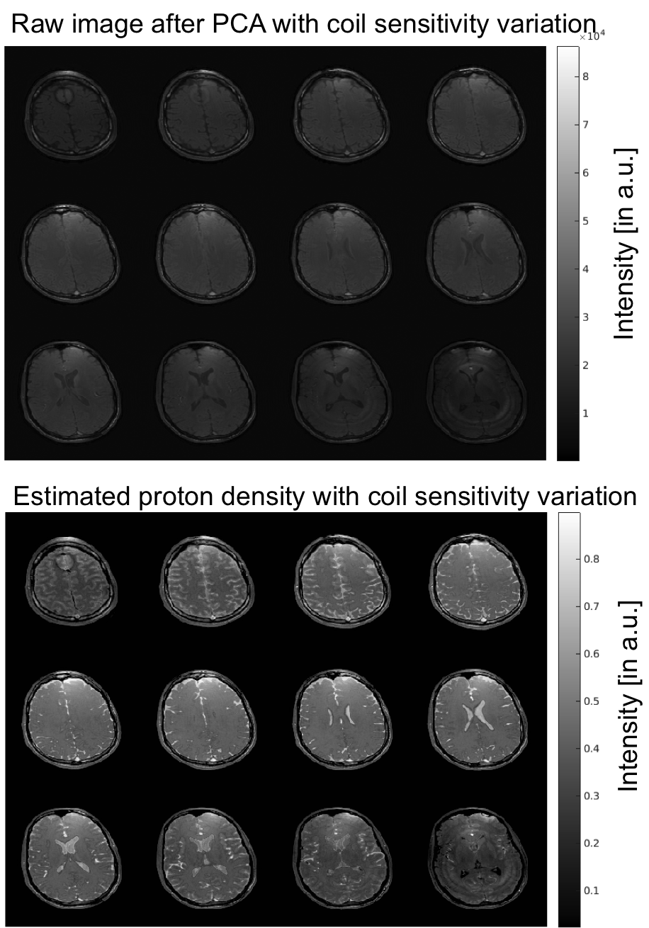
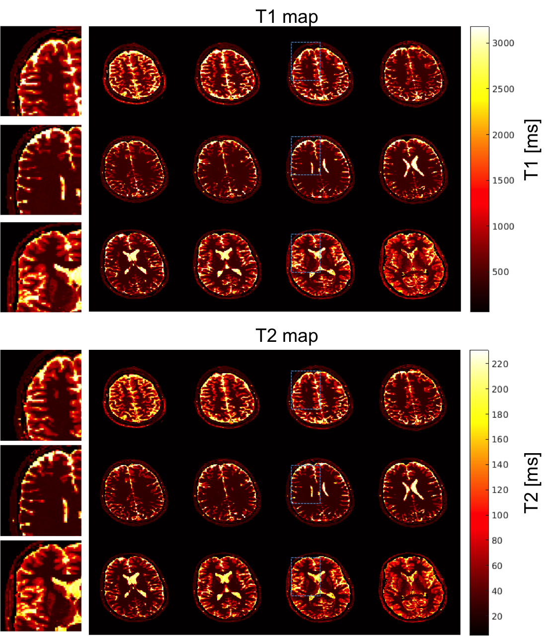
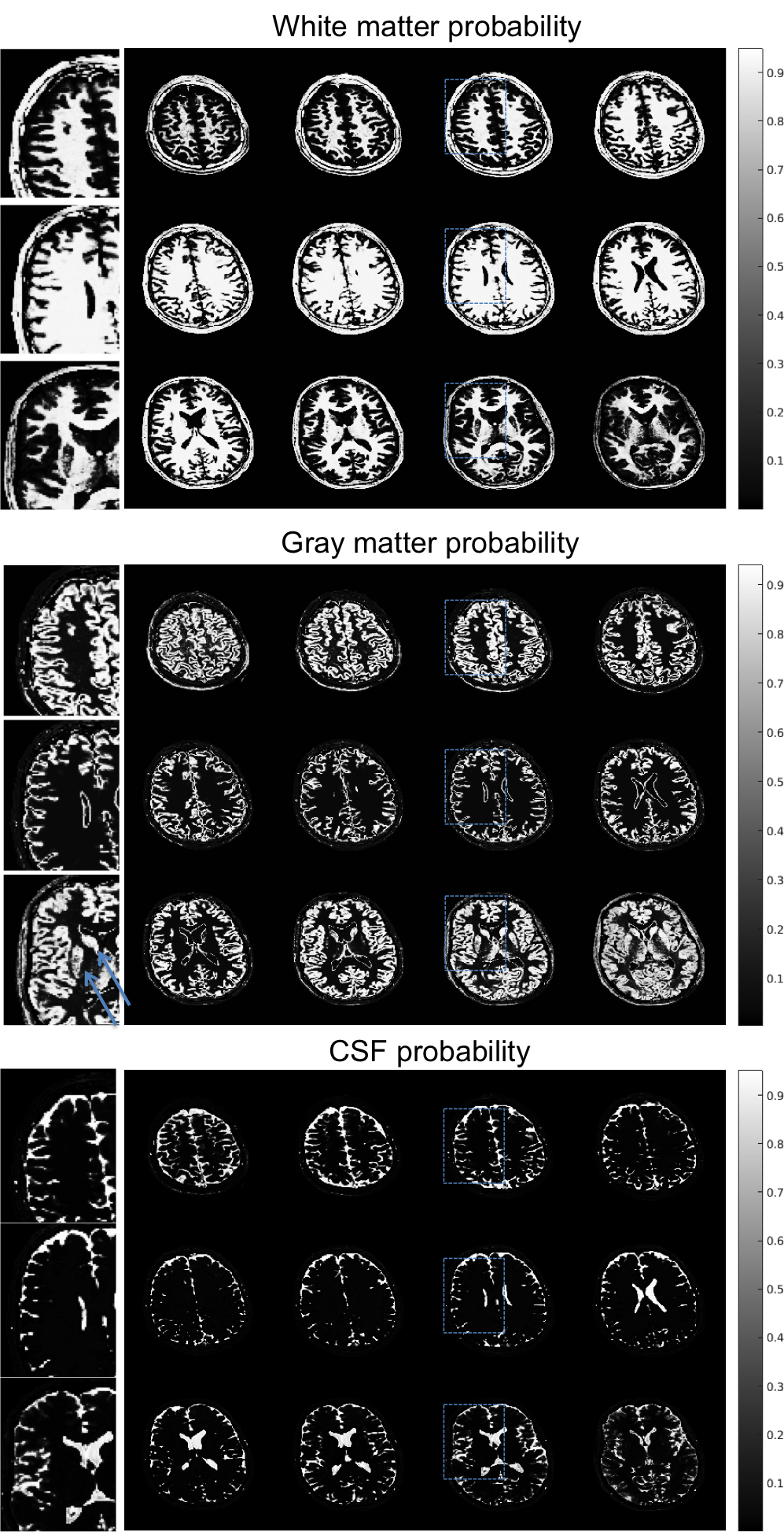
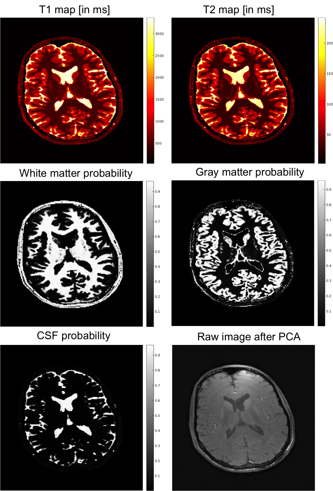
Figure 2 shows the coil sensitivity weighted proton density map (Fig. 2 bottom) estimated from the in vivo images (Fig. 2 top). These images contained the effects of varied coil sensitivity profiles and imperfect slice selection. However, these variations were decoupled from the T1 and T2 maps and segmentation results. In Figure 3, the estimated T1 and T2 maps were in accordance with known brain anatomy, and showed no systemic bias due to the coil sensitivity variation. The estimated T1 and T2 values were slightly lower than the literature values ^13,14.This could be caused by the magnetization transfer (MT) effect . In Figure 4, excellent whole brain segmentation was demonstrated, using the direct output of neural network (in probability sense). Especially, the deep brain gray matter nuclei, e.g. caudate nucleus and putamen, which are typically challenging for segmentation methods, were well recognized by the deep neural network. Some partial volume effects on the interface between gray matter and CSF was noticed in Fig. 4. However, the probably masks provide excellent information on the location and extent of partial volume effects, and could possibly be used to correct the parameter estimation for these regions. Fig. 5 shows a summary of relaxometry/segmentation results for one slice.

Discussion

In this study, simultaneous relaxometry and segmentation of in vivo human brain was performed within seconds using a trained deep neural network with 6 fully connected layers. Further development of even advanced neural networks with a similar training procedure and architecture could potentially perform more complex tasks, e.g., the segmentation/quantification/recognition of anatomical changes in pathological brains and other organs.

Conclusion

In conclusion, deep neural network can directly generate brain T1 and T2 maps in conjunction with the segmentation of gray matter, white matter and CSF.

Acknowledgements

We receive grant supports (NIH R56HL133663 and NIH R21NS089004) from NIH.

References

1. Alexander, A. L. et al. Characterization of cerebral white matter properties using quantitative magnetic resonance imaging stains. Brain Connect. 1, 423–46 (2011).

2. Deoni, S. C. Magnetic resonance relaxation and quantitative measurement in the brain. Methods Mol Biol 711, 65–108 (2011).

3. Laule, C. et al. Magnetic Resonance Imaging of Myelin. Neurotherapeutics 4, 460–484 (2007).

4. Tofts, P. Quantitative MRI of the Brain: Measuring Changes Caused by Disease. Quantitative MRI of the Brain Measuring Changes Caused by Disease (2005). doi:10.1002/0470869526

5. Chai, J.-W. et al. Quantitative analysis in clinical applications of brain MRI using independent component analysis coupled with support vector machine. J. Magn. Reson. Imaging 32, 24–34 (2010).

6. West, J., Warntjes, J. B. M. & Lundberg, P. Novel whole brain segmentation and volume estimation using quantitative MRI. Eur. Radiol. 22, 998–1007 (2012).

7. West, J., Blystad, I., Engström, M., Warntjes, J. B. M. & Lundberg, P. Application of Quantitative MRI for Brain Tissue Segmentation at 1.5 T and 3.0 T Field Strengths. PLoS One 8, (2013).

8. Sled, J. G. & Pike, G. B. Quantitative imaging of magnetization transfer exchange and relaxation properties in vivo using MRI. Magn. Reson. Med. 46, 923–931 (2001).

9. Yarnykh, V. L. Fast Macromolecular Proton Fraction Mapping from A Single Off-Resonance Magnetization Transfer Measurement. 178, 166–178 (2012).

10. Yarnykh, V. L. Time-Efficient , High-Resolution , Whole Brain Three-Dimensional Macromolecular Proton Fraction Mapping. 2106, 2100–2106 (2016).

11. Mezer, A. et al. Quantifying the local tissue volume and composition in individual brains with magnetic resonance imaging. Nat. Med. 19, 1667–72 (2013).

12. Ma, D. et al. Magnetic resonance fingerprinting. Nature 495, 187–92 (2013). 13. Wansapura, J. P., Holland, S. K., Dunn, R. S. & Ball, W. S. NMR Relaxation Times in the Human Brain at 3 . 0 Tesla. 538, 531–538 (1999).

14. Wright, P. J. et al. Water proton T1 measurements in brain tissue at 7, 3, and 1.5 T using IR-EPI, IR-TSE, and MPRAGE: results and optimization. MAGMA 21, 121–130 (2008).

15. Liu, J. & Saloner, D. Accelerated MRI with CIRcular Cartesian UnderSampling ( CIRCUS ): a variable density Cartesian sampling strategy for compressed sensing and parallel imaging. 4, 57–67 (2014).

16. Liu, J., Haraldsson, H., Feng, L. & Saloner, D. Free-Breathing Whole Heart CINE Imaging with Inversion Recovery Prepared SSFP Sequence: Feasibility for Myocardium Viability Assessment. ISMRM Proceeding #2410, (2014).

17. Kingma, D. P. & Ba, J. L. ADAM: A Method for Stochastic Optimization. Int. Conf. Learn. Represent. (2015).

Figures

Figure 1 (a) Proposed method assumed the feasible parameter space can be divided into boxes that were binary labeled for white matter (WM), gray matter (GM), and cerebrospinal fluid (CSF). (b) A deep neural network was used to perform pixel-wise estimation of T1, T2, and WM, GM and CSF probabilities. Each input pixel contained coefficients of 6 principal components from a principal component analysis (PCA) preprocessing. The neural network was trained with T1 and T2 drawn from the parameter feasibility region as well as varied proton density weightings (0% to 100%), varied noise levels (0% to 10%), and binary class labels (in Fig. a)

Figure 2 (top) Raw image of the first principal component contained varied coil sensitivity profiles and imperfect slice selection. 12 out of 30 slices are shown. (bottom) The coil sensitivity weighted proton density was estimated together with the relaxometry and segmentation; this setting made the proposed method highly tolerant of varied coil sensitivity profiles and also to some extent the imperfect slice selection.

Figure 3 In vivo 3D T1 and T2 estimation for the raw image data in Fig. 2. Noticed that the proposed method highly tolerated varied coil sensitivity profiles and to some extent the imperfect slice selection (in Fig. 2). 12 out of 30 slices are shown.

Figure 4 Whole brain segmentation was the direct output of neural network in conjunction with the relaxometry results in Fig. 3. 12 out of 30 slices are shown. Noticed that the proposed method in particular is robust in segmenting the deep gray matter nuclei, e.g. caudate nucleus and putamen (arrows). The probability means the likelihood of a pixel to contain a tissue/fluid type.

Figure 5 Summary of relaxometry and segmentation results for one slice. The estimated maps agreed well with brain anatomy.

Proc. Intl. Soc. Mag. Reson. Med. 26 (2018)

0658