Introduction

Studying the rhesus brain development based on Magnetic Resonance (MR) images is important not only for understanding the maturation of normal brains, but also for investigating the intervention and treatment of neurodevelopmental disorders^1,2. However, available adult monkey brain atlases are not suitable for the studies during the early postnatal stage. This is because the MRI of infant rhesus brains have dramatic changes in image contrast, intensity, appearance and folding degree across different ages. Therefore, for the first time, we developed the spatiotemporal (4D) cortical surface atlas of infant rhesus macaques to comprehensively characterize the early postnatal brain development. Specifically, our 4D macaque atlas was created at 13 time-points, from 2 weeks to 24 months of age, using 138 serial MRI scanned for 32 rhesus monkeys. In addition, we further parcellated our 4D atlas into distinct regions purely based on the cortical developmental trajectories. Our parcellation results can reflect the underlying cortical cytoarchitectonic changes and thus help define the microstructurally distinctive cortical regions.

Methods

This study was performed based on a public rhesus macaque neurodevelopment dataset with 32 rhesus monkeys, in which each monkey has 4 to 5 longitudinal MRI scans during early postnatal stages with acquisition parameter detailed in¹. We applied our in-house developed tools for infant brain tissue segmentation and cortical surface reconstruction^3-5. All cortical surfaces were then mapped onto a standard sphere to facilitate atlas construction and analysis, with each vertex attached with cortical morphological features (e.g., cortical thickness, sulcal depth, average convexity, and curvature). Directly building the 4D cortical surface atlas using group-wise surface registration to align all subjects at different ages separately would result in temporally-inconsistent atlases, which may influence the analysis of early brain development. To tackle this challenge and leverage the within-subject longitudinal constraints, an advanced registration strategy⁴ was adopted in this study. Specifically, we first performed the intra-subject registration to obtain within-subject mean cortical surfaces. Then, we performed the inter-subject registration of within-subject mean surfaces to obtain unbiased and longitudinally-consistent 4D cortical surface atlases. Based on the established longitudinal and cross-sectional cortical correspondences, the developmental trajectory was defined at vertex-level by concatenating the corresponding cortical attributes across different time-points. The Pearson’s correlation was computed between any two vertices, forming a similarity matrix for each subject. This matrix was then normalized to [0, 1] and averaged across different subjects. We then applied the spectral clustering method⁶ on the averaged similarity matrix to perform the parcellation. We used the local surface area in this study for atlas parcellation, which, however, can be easily replaced by other cortical attributes, e.g., cortical thickness and cortical folding.

Results

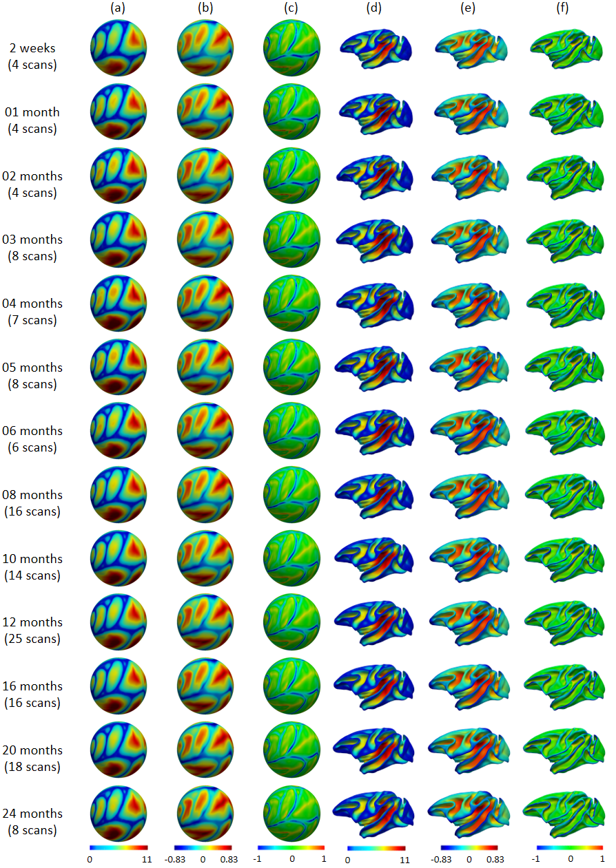
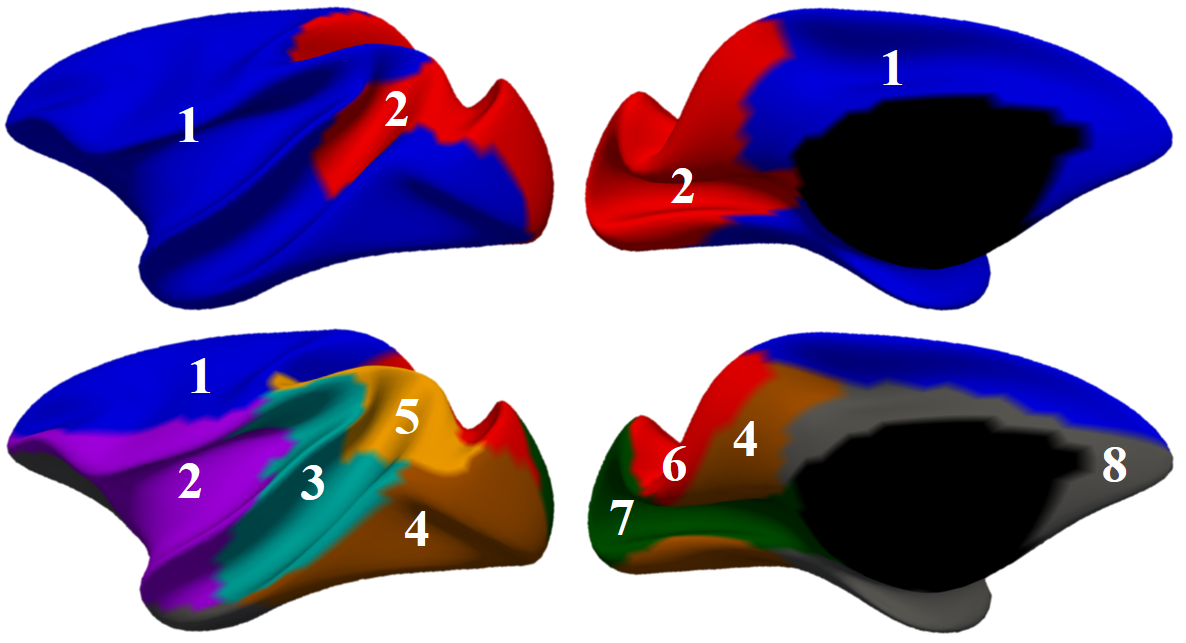
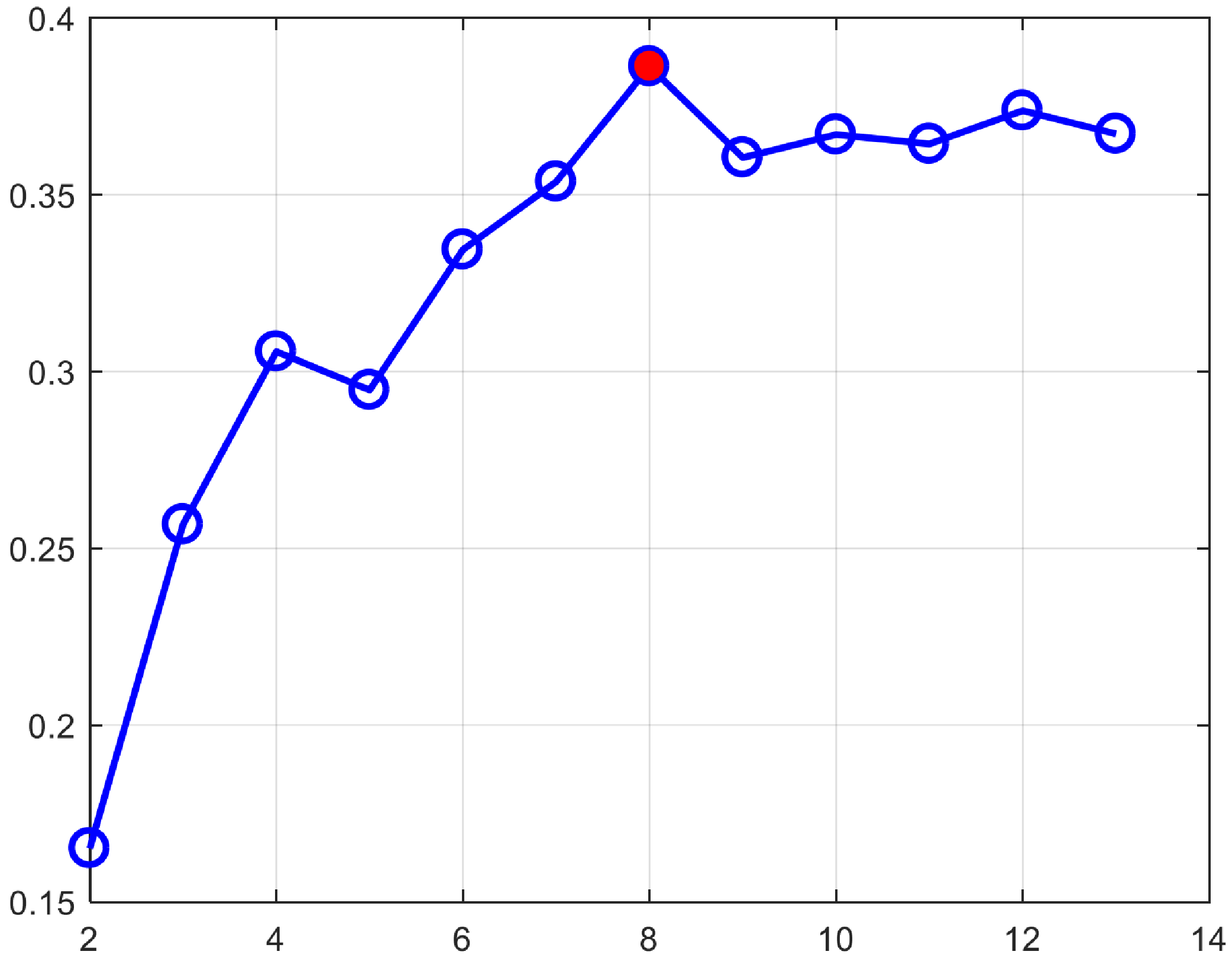
Fig. 1 shows our constructed 4D cortical surface atlas of rhesus macaques during the first 24 months, including 13 time-points at 2 weeks, 1, 2, 3, 4, 5, 6, 8, 10, 12, 16, 20 and 24 months of age. We can observe that major cortical folds are well established since birth and remain relatively stable during brain development. However, both average convexity and sulcal depth develop rapidly during the first 6 months, and then change gradually. These observations indicate the necessity of building an age-specific atlas, especially for early postnatal stage undergoing dynamic development. To capture the main pattern in developmental regionalization of the cortical structure, we first show the two-cluster parcellation map (top row of Fig. 2), which identifies a clear anterior-posterior division. To determine an appropriate number of clusters, we computed the widely used silhouette coefficient⁷. As shown in Fig. 3, according to the peak of the silhouette coefficients, we identified 8 clusters and presented the parcellation map in the bottom row of Fig. 2, from which we can observe that the obtained clusters are consistent with structurally and functionally meaningful regions. According to the labeled numbers in the figure, these regions approximately correspond to: (1) superior and middle frontal, (2) inferior frontal, insula, and temporal pole, (3) superior temporal, (4) inferior temporal and precuneus, (5) supra-marginal, (6) superior parietal, (7) occipital, and (8) limbic and cingulate. This parcellation map shows meaningful correspondences to existing neuroscience knowledge.

Conclusion

We have built the first 4D cortical surface atlas for infant rhesus monkeys aged from 2 weeks to 24 months, with dense time points and in an unbiased and longitudinally-consistent manner. We have also unprecedentedly parcellated our 4D cortical surface atlas into distinct regions using developmental trajectories of local surface area. Our 4D atlas equipped with development-based parcellation maps will be a good reference for visualization, spatial normalization, analysis and comparison among various studies on both normal and abnormal monkey brain development.

Acknowledgements

This work was partially supported by NIH grants (MH108914 and MH107815). We thank Dr. Matin A. Styner and his co-authors for making the UNC-Wisconsin Neurodevelopment Rhesus MRI Database publicly available.