0642
Validating and Measuring Transfer Functions of Straight Wires using a Combination of an Electro-optic Field Sensor and Simulation1Department of Radiology, Medical Physics, Medical Center - University of Freiburg, Faculty of Medicine, University of Freiburg, Freiburg, Germany, 2German Consortium of Translational Cancer Research Freiburg Site, German Cancer Research Center (DKFZ), Heidelberg, Germany, 3BIOLAB Technology AG, Zürich, Switzerland
Synopsis
To investigate deep brain stimulators, pacemakers or other elongated structures the transfer function was proposed to characterize these devices. A electro-optic E-field sensor is used to acquire 2D field data of copper wires excited at one tip for 64 and 123MHz. The data is compared to simulations and transfer functions are calculated from these simulations. These are compared to experimentally acquired transfer functions.
Introduction
Due to the increased use of pacemakers, deep brain stimulator (DBS), and other implanted active and passive devices, methods are currently developed and validated to study the response of active devices to the radio-frequency fields in the MR environment. In particular, the interaction of the elongated structures with the incident RF field can lead to dangerous temperature increases up to 60°C1, and safety measures need to be taken to ensure patient safety1,2 .To characterize the response to an arbitrary incident electric RF field, the transfer function approach has been proposed, and methods to measure the transfer function have been described3,4,5 which are based on electrical coupling to the implant (e.g., with a small dipole antenna). In this work, an electro-optical sensor is used to measure the transfer function, based on electro-optical sampling which benefits from sub-millimeter spatial resolution, high SNR and no metallic induced field-interaction6. To demonstrate feasibility, the measured E-field distribution of a straight wire excited by a monopole antenna was validated via simulations and sampling for determining transfer functions is investigated and compared with simulations.Methods
The electro-optic E-field sensor is based on the Pockels effect where the polarization of a laser beam becomes modulated proportional to an external electric field when passing through an electro-optical medium (LiNbO3) and by evaluation of the polarization state, the E-field is reconstructed6. The 1x1x1mm³ electro-optic crystal is mounted on the tip of a non-metallic sensor probe. Spatially resolved field scans are achieved by sweeping the probe along the x- and y-direction by a motor driven translation stage. According to the crystal orientation the laser light is polarized to the normal component of the E-field.4 samples/s of data were acquired during the scan. Single wires with different lengths (L=10cm, 20cm, 30cm) made of pure copper and Polyurethan isolation (1cm removed at both ends) were placed in distilled water ($$$\epsilon_r = 81$$$, $$$\sigma = 5.5\cdot10^-6\,S/m$$$). The wires were excited at one tip by a small monopole and the resulting Ez-field was measured with a resolution of 1x1mm2 in an area of 2cm around the wire for proton frequencies of 1.5 T and 3 T (i.e., 64 and 123 MHz) at a height of 1mm above the wire. For comparison, simulations were performed with the finite-difference time domain software Sim4Life Version 3.4 (ZMT AG, Zürich, Switzerland). The 10cm long semi-rigid coaxial cable and the excitation source were modeled with a voltage source driving the coaxial cable. Simulation time was between 1 and 1.5 hours per setting (using GPU acceleration). For simulations and measurements background subtraction was applied, simulating and measuring the setup without a cable present and subtracting from the results. From this the transfer function was calculated via Ampere’s law from simulation data. In order to determine the transfer function experimentally, the sensor remained stationary at one end of the 20cm long wire, while the excitation source was moved along the sample. Each data point was normalized relative to the magnitude of the of the excitation field
Results
The measurement times of the E-field measurements for 10cm, 20cm and 30cm were 35min, 48min, and 62min for 1x1mm2 resolutions. Single line measurements were performed below 2min. Figure 2 shows the E-field at f = 64 MHz and 128 MHz next to the simulation results. The theoretical dipole behavior of the structure was confirmed, and higher harmonics for the 30cm wire, which is above the resonance length of 123MHz in distilled water, is present in both simulations and measurements. The calculated transfer function (Figure 3) is in good agreement for the measured case of the 20cm wire as well as with the literature3.Discussion
In general, transfer functions derived from the E-field measurements are in good agreement with the simulations - observed differences can be attributed to uncertainties in material parameters and dimensions. The current study is only based on the measurement of the z component since the measurements are performed in the vicinity of the sample where the E-field is perpendicular to conducting structures.The presented setup is able to validate E-field distributions and transfer functions within relatively short measurement times, and it does not need electrically conducting elements such as dipoles, which can cause additional systematic errors. The applications of electro-optical electric field measurements are optimization of RF coils, safety assessment of active and passive devices, and general field measurements for diagnostic purposes.
Acknowledgements
References
1. Yeung CJ, Susil RC, Atalar E. RF safety of wires in interventional MRI: Using a safety index. Magn. Reson. Med. 2002;47:187–193. doi: 10.1002/mrm.10037
2. Zeng X, Barbic M, Chen L, Qian C. Sensitive enhancement of vessel wall imaging with an endoesophageal Wireless Amplified NMR Detector (WAND): Integrated Endoesophageal Detector with a Wirelessly Powered Amplifier. Magn. Reson. Med. 2017;78:2048–2054. doi: 10.1002/mrm.26562
3. Tokaya J p., Raaijmakers A j. e., Luijten P r., Bakker J f., van den Berg C a. t. MRI-based transfer function determination for the assessment of implant safety. Magn. Reson. Med. 2017:n/a-n/a. doi: 10.1002/mrm.26613
4. Missoffe A, Aissani S. Experimental setup for transfer function measurement to assess RF heating of medical leads in MRI: Validation in the case of a single wire: Transfer Function Measurement Setup. Magn. Reson. Med. [Internet] 2017. doi: 10.1002/mrm.26773
5. Feng S, Qiang R, Kainz W, Chen J. A Technique to Evaluate MRI-Induced Electric Fields at the Ends of Practical Implanted Lead. IEEE Trans. Microw. Theory Tech. 2015;63:305–313. doi: 10.1109/TMTT.2014.2376523
6. Reiss S, Bitzer A, Bock M. An optical setup for electric field measurements in MRI with high spatial resolution. Phys. Med. Biol. 2015;60:4355–4370. doi: 10.1088/0031-9155/60/11/4355
Figures
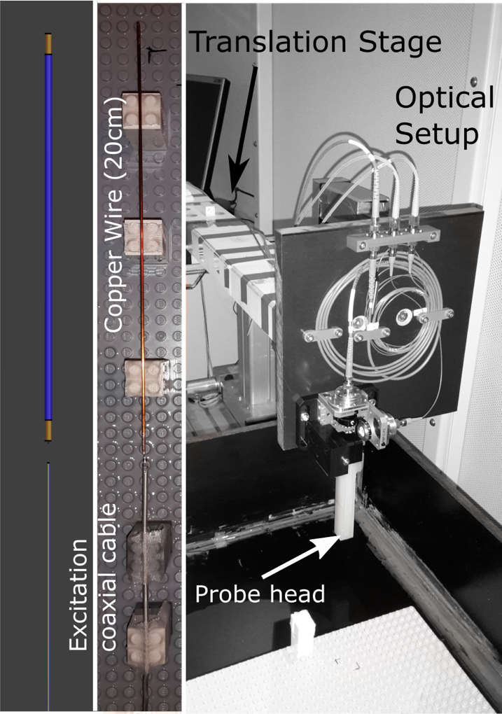
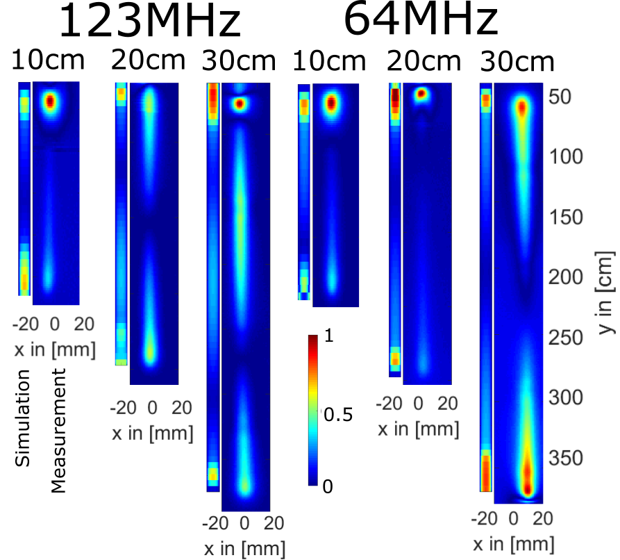
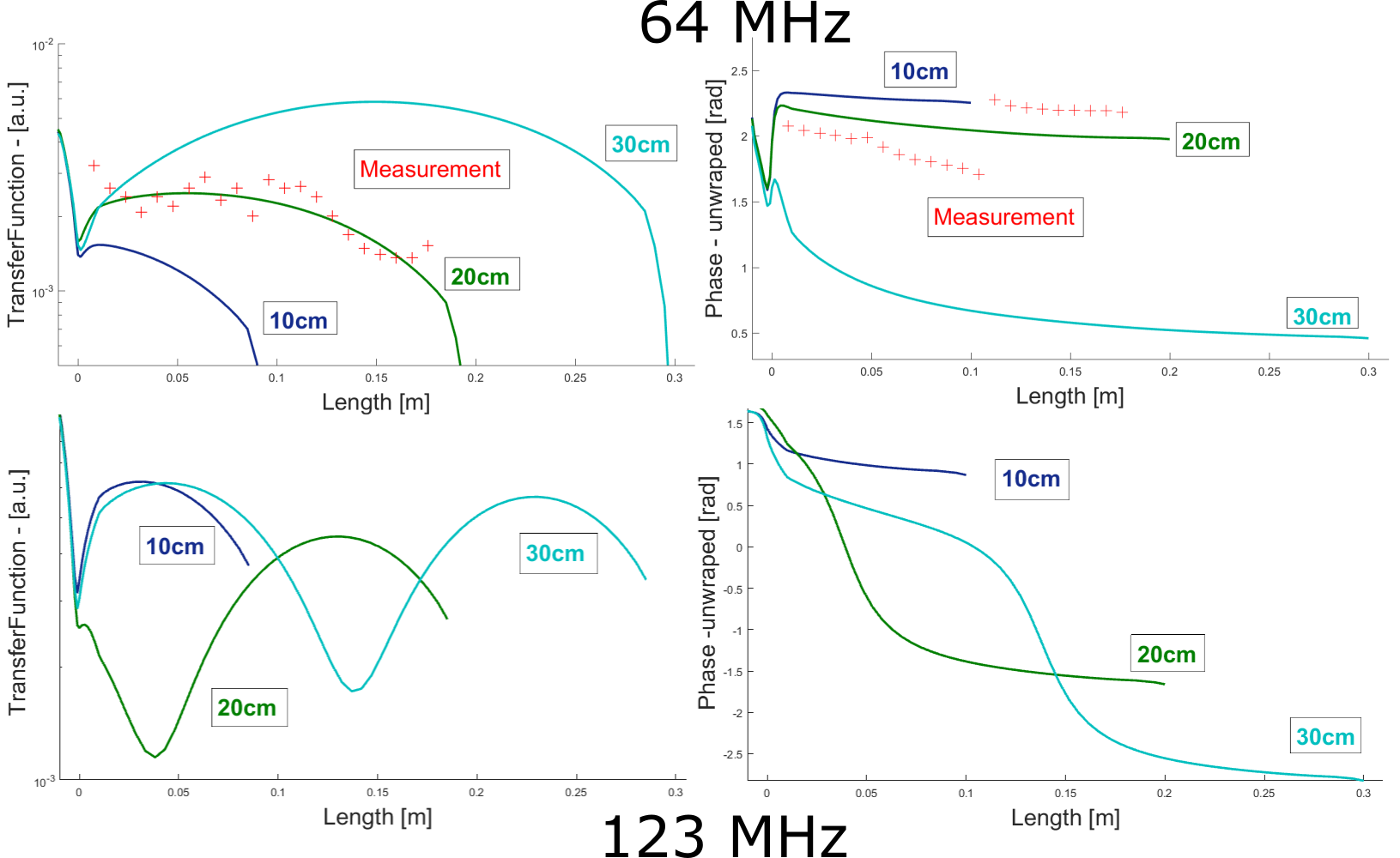
Figure 3: Magnitude (on a logarithmic scale) and phase of the simulated transfer functions at 64MHZ and 123MHz for different wires; the dip marks the excitation probe marks due to the background subtraction, the measured transfer function is shown in red