0641
Sensitivity analysis of Peripheral Nerve Stimulation modeling: Which model parameters actually matter?1Computer Assisted Clinical Medicine, Medical Faculty Mannheim, Heidelberg University, Mannheim, Germany, 2A. A. Martinos Center for Biomedical Imaging, Department of Radiology, Massachusetts General Hospital, Charlestown, MA, United States, 3Harvard Medical School, Boston, MA, United States, 4Harvard-MIT Division of Health Sciences and Technology, Cambridge, MA, United States
Synopsis
Peripheral nerve stimulation (PNS) has become the main limitation for MRI with high-performance gradients. Recently, we proposed a simulation framework to predict PNS thresholds for arbitrary coil geometries to directly address PNS considerations during the coil prototyping phase. In order to ensure robust modeling of PNS (and thus convergence of the coil optimization phase), we analyze the sensitivity of our framework to key simulation parameters such as the temporal and spatial resolution of the induced electric fields, dielectric tissue parameters of our body models, and the location of the neurodynamic model compartments along the nerve fibers.
Target audience
MR safety researchers, MRI gradient designers.Purpose
Peripheral nerve stimulation (PNS) is a major limitation of fast imaging in MRI1,2. Recently, we proposed a simulation framework that allows for numerical prediction of PNS thresholds for arbitrary coil geometries using realistic body models in conjunction with neurodynamic models3. We demonstrated the applicability of our framework to leg/arm stimulation experiments3,4 and whole-body MRI gradient coils5. Numerical prediction of PNS may allow for computational optimization of gradient coils with potentially increased PNS thresholds without the need to build expensive prototype coils. For coil optimization to converge, it is crucial that the PNS prediction is robust and accurate. In this work, we address the question of which parameters in the PNS simulation framework have the highest impact on PNS prediction accuracy and what are sufficient values for resolution and time-step size.Methods
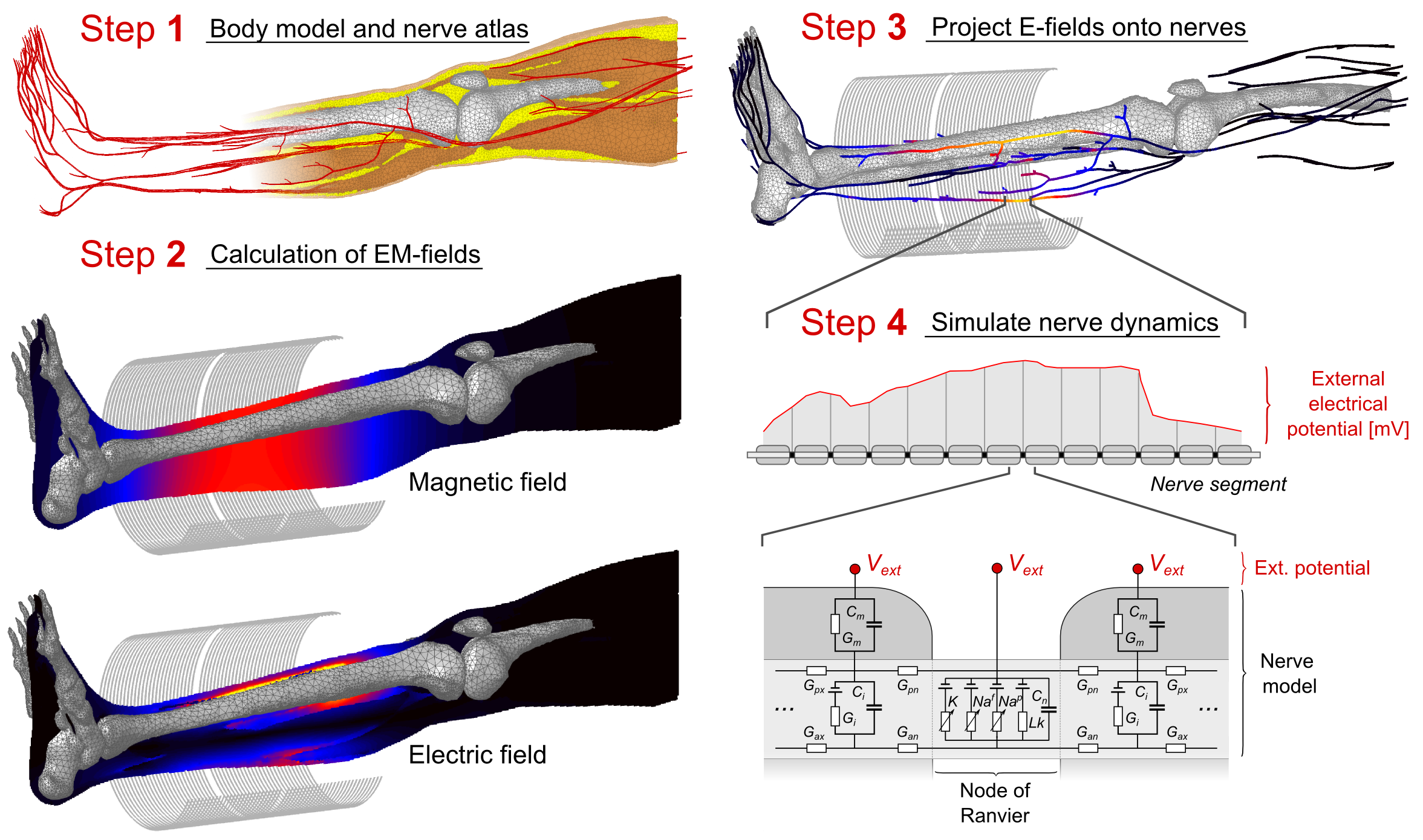
PNS prediction workflow: To simulate PNS, we first compute the EM fields created by the coil in a detailed body model (Fig. 1, Steps 1 and 2). We then superimpose an atlas of nerve fibers to sample the induced E-fields to obtain electric potential changes along the nerves (Step 3). These are modulated in time by the coil’s driving waveform and fed into the MRG neurodynamic model6 to simulate the nerve response (Step 4), including possible action potentials that indicate PNS. The process is repeated for different modulation frequencies (sinusoidal and trapezoidal) to generate a threshold curve.
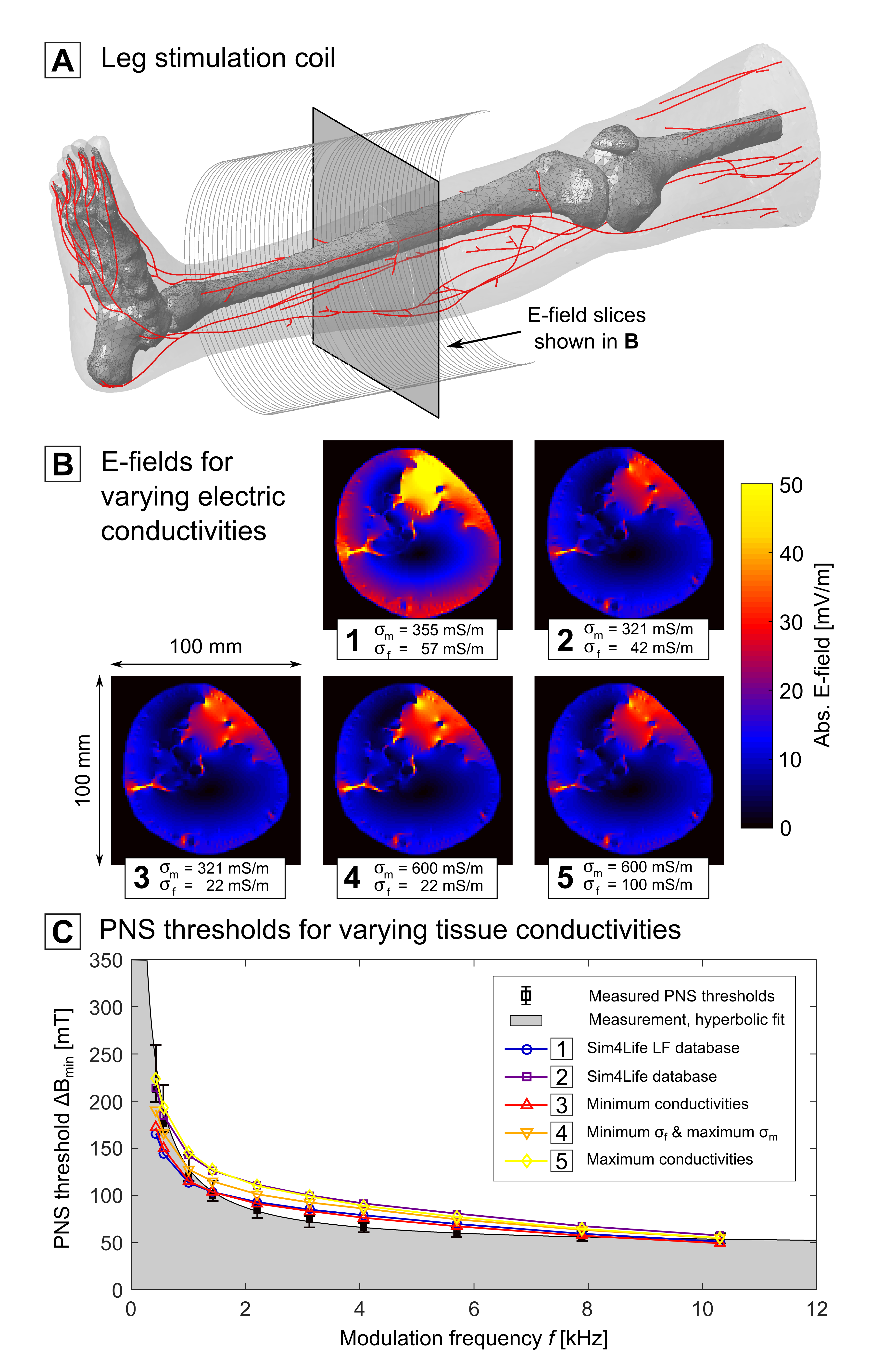
Dielectric tissue properties: We computed the E-field distribution in the body with Sim4Life’s (Zurich MedTech AG, Switzerland) hexahedral magneto-quasistatic FEM solver using varying electric tissue conductivities for muscle (σm=321…600 mS/m7,8) and fat (σf=22…100 mS/m7,9) to study their influence on the PNS threshold.
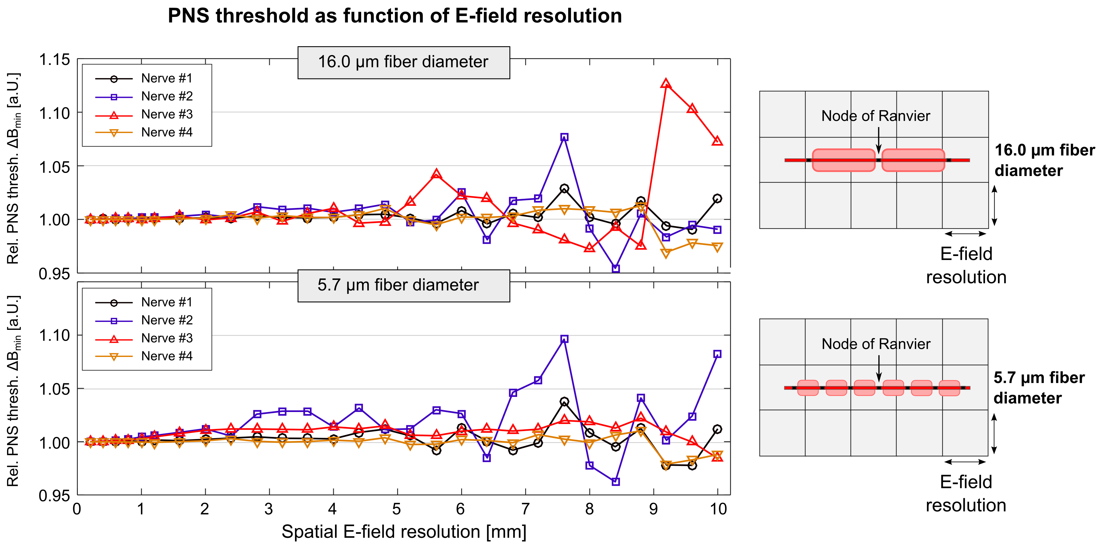
E-field resolution: We varied the spatial E-field resolution between 0.2 mm and 10.0 mm by subsampling the map and computed PNS threshold curves using nerves with large (16.0 µm) and small (5.7 µm) fiber diameters to determine the sensitivity of the PNS threshold to the field resolution.
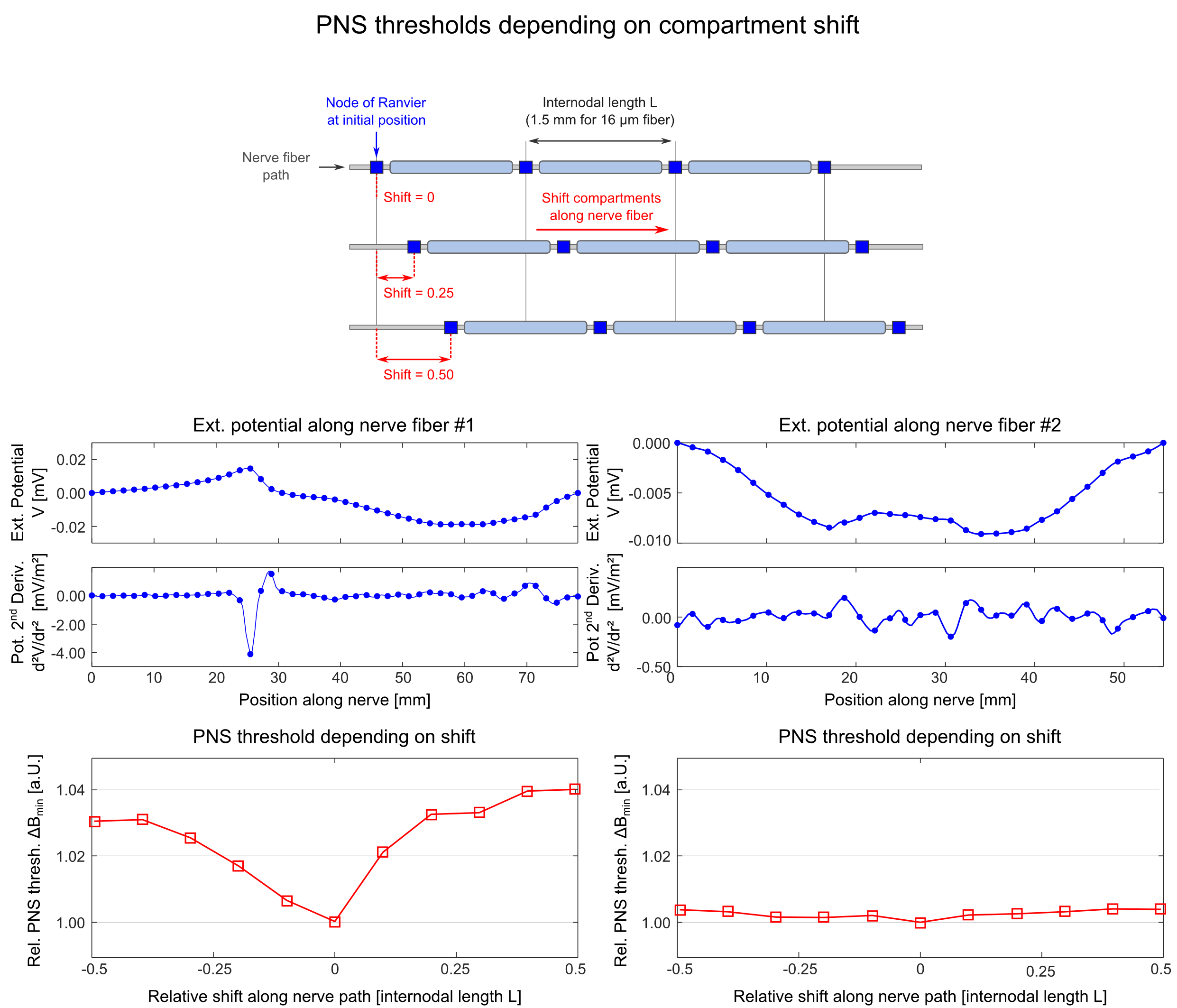
Position of nerve model compartments: The MRG neurodynamic model is based on a double cable circuit model that consists of electric compartments placed along the nerve path at fixed spacing. We investigated the effect of shifting the entire compartment model along the nerve path (while maintaining the spacing between compartments).
Temporal resolution: The MRG model requires numerically solving a set of coupled differential equations using discrete time-steps. For each modeled gradient waveform, we increased the time-step to determine its effect on the PNS thresholds. Like the spatial resolution, the coarsest temporal resolution needed for accurate threshold prediction is desirable for decreasing simulation times ultimately allowing more gradient configurations to be evaluated.
Results
Figure 2 shows E-field maps of the leg stimulated by a solenoid coil (A) for varying electric conductivities of muscle and fat. The different tissue conductivities influence the E-field distribution (B), leading to a variation of the PNS threshold curves comparable to the experimental variability (C).
Figure 3 shows the PNS thresholds for 16.0 µm (top) and 5.7 µm fibers (bottom) as a function of spatial E-field resolution. Large diameter fibers seem slightly less sensitive to the E-field resolution than small fibers, likely due to their larger separation between nodes of Ranvier. However, a resolution of 1 mm is sufficient for both small and large fiber diameters.
Figure 4 shows the effect of shifting the MRG model compartments along the nerve fiber for two exemplary nerves (1st/2nd row: electric potential and its second derivative along the nerve; 3rd row: PNS threshold as a function of compartment shift). We found that nerves that are stimulated locally are more sensitive to the nerve model compartment locations (PNS variation 4%, left column) than nerves that are stimulated in a broader region (PNS variation 0.5%, right column). It is not straightforward to determine the location of the model compartments (“shift value”) that leads to the most conservative PNS threshold. We therefore evaluate each nerve at multiple shift locations.
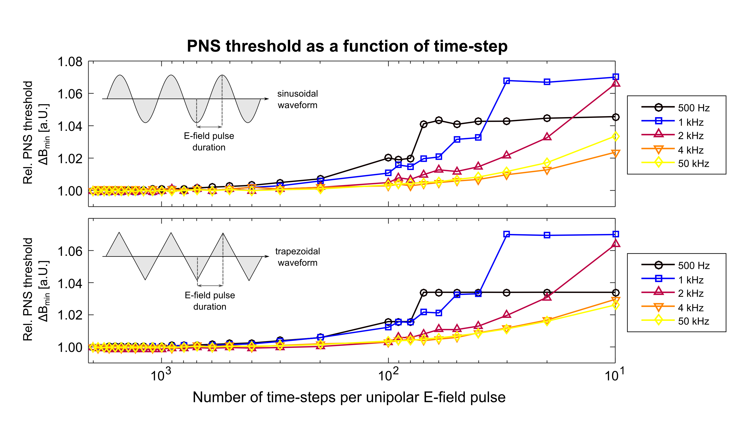
Figure 5 shows PNS thresholds for sinusoidal (top) and trapezoidal waveforms (bottom), plotted as a function of the time-step used to solve the MRG model differential equations. We found 500 time-steps per gradient wave ramp is sufficient for accurate prediction of PNS thresholds. However, the time-step should not exceed 2 µs to ensure that the nerve membrane dynamics are modeled correctly.
Conclusion
We found that modest spatial-temporal resolutions are sufficient for accurate PNS prediction. The simulation framework is moderately sensitive to dielectric tissue parameters and nerve positions, but these can likely be controlled to yield values within the variance of a population.Acknowledgements
No acknowledgement found.References
[1] McNab et al., “The Human Connectome Project and beyond: Initial applications of 300 mT/m gradients”. NeuroImage 80, 2013.
[2] Setsompop et al., “Pushing the limits of in vivo diffusion MRI for the Human Connectome Project”. NeuroImage 80, 2013.
[3] Davids et al., “Predicting magnetostimulation thresholds in the peripheral nervous system using realistic body models”. Sci. Rep. 7:5316, 2017.
[4] Saritas et al., “Magnetostimulation limits in magnetic particle imaging”. IEEE TMI 32(9), 2013.
[5] Davids et al., “Simulation of peripheral nerve stimulation thresholds of MRI gradient coils”. ISMRM proceedings, 2018.
[6] McIntyre et al., “Modeling the excitability of mammalian nerve fibers: Influence of afterpotentials on the recovery cycle”. J Neurophysiol. 87(2), 2002.
[7] Gabriel et al., “The dielectric properties of biological tissues: III. Parametric models for the dielectric spectrum of tissues”. Phys. Med. Biol. 41, 1996.
[8] Rush et al., “Resistivity of body tissues at low frequencies”. Circ. Res. 12, 1963.
[9] Gabriel et al., “Electrical conductivity of tissue at frequencies below 1 MHz”. Phys. Med. Biol. 54, 2009.
Figures