Synopsis

Annihilating filter-based low rank Hankel matrix approach (ALOHA) was recently used as a reference-free ghost artifact correction method. Inspired by another discovery that convolutional neural network can be represented by Hankel matrix decomposition, here we propose a deep CNN for reference-free EPI ghost correction. Using real EPI experiments, we demonstrate that the proposed method effectively removes the ghost artifacts with much faster reconstruction time compared to the existing reference-free approaches.

Introduction

Theory

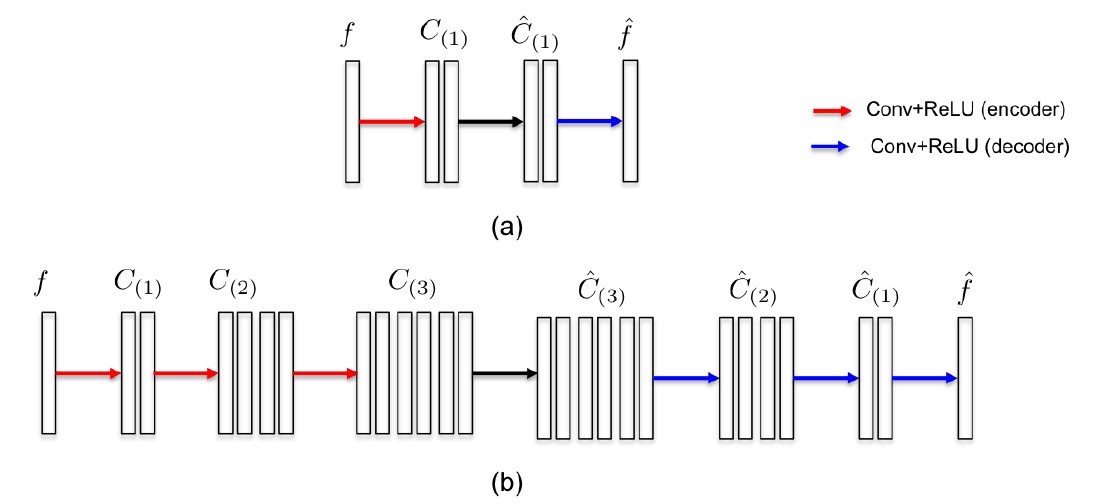
As an intriguing extension of ALOHA, it was recently shown that a CNN is closely related to Hankel matrix decomposition⁶. Let $$$f\in R_n $$$ denote an input signal. Then, for a given Hankel matrix $$$H(f)\in R_{n \times d} $$$, let $$$\phi$$$ and $$$\tilde{\phi}\in R_{n \times m}$$$ (resp. $$$\psi$$$ and $$$\tilde{\psi}\in R_{d \times q}$$$) are frame and its dual frame, respectively, satisfying the frame condition: $$$\tilde{\phi}\phi^T =I$$$, $$$\psi\tilde{\psi}^T =I$$$ such that it decompose the Hankel matrix: $$H(f) = \tilde{\phi}\phi^T H(f) \psi\tilde{\psi}^T = \tilde{\phi}C\tilde{\psi}^T~~(1)$$ One of the most important discoveries in [6] is to reveal that (1) can be equivalently represented in the signal domain using convolutional framelets expansion, where $$$C$$$ is the framelet coefficient matrix obtained from the encoder part of convolution: $$C=\Phi^T (f \ast \bar{\Psi})~~~(2)$$ and the decoder-part convolution is given by $$f = (\tilde{\Phi}C)\ast \tau(\tilde{\Psi})~~~(3)$$ Here, $$$\bar{\Psi}, \tau(\tilde{\Psi})$$$ are realigned vector from $$$\Psi,\tilde{\Psi}$$$, respectively⁶. The simple convolutional framelet expansion using (2) and (3) is so powerful that a CNN with the encoder- decoder architecture emerges from them by recursively inserting multiple pairs of (2) and (3) between the pair as shown, for example, in Fig. 1 for the case of $$$\Phi=I$$$. Then, a deep CNN training can be interpreted to learn the basis matrix $$$\Psi$$$ for a given basis $$$\Phi$$$ such that maximal energy compaction can be achieved. For more detail, see [6].

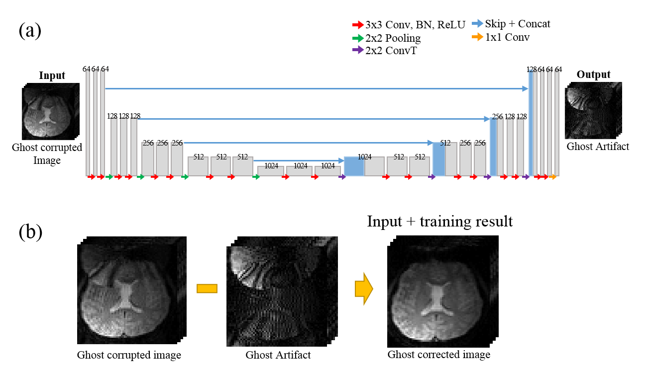
Here, the global basis matrix $$$\Phi$$$, which are multiplied from the left of $$$H(f)$$$, interacts with all input signals to capture global signal distribution of the input signal. Thus, the choice of the global basis is important in designing a deep network. Since the ghost artifacts are distributed globally due to the even-odd line phase mismatch, we choose the low-pass branch of Haar wavelet basis. Interestingly, this results in U-net like encoder-decoder architecture as shown in Fig. 2(a).

Methods

Fig.2(a) illustrates the proposed encoder-decoder network architecture. After estimating the ghost component, a ghost corrected image is obtained by subtracting the artifact from corrupted EPI image as shown in Fig.2(b).

We used 30 slices of GRE(gradient-echo)-EPI data with 12 coils. For fMRI experiments, 60 temporal frames were obtained. This data set were acquired using conventional EPI sequence with a Siemens 3T whole body MR scanner. The data acquisition parameters were as follows: TR/TE = 3000/30 ms, 3mm slice thickness, FOV of 240x240mm2, and 64x64 matrix size with full Fourier sampling. Among this data, 27 z-slice data was used for training and the remaining 3slices were used as for validation. For fMRI experiments, this training and validation was performed for a single temporal frame, and the trained network was used for the remaining 59 frames. Because ALOHA-based correction provided the best ghost removal result, we used the ALOHA-based ghost-correction images as the ground-truth images, and the label database was constructed accordingly.

Results&Discussion

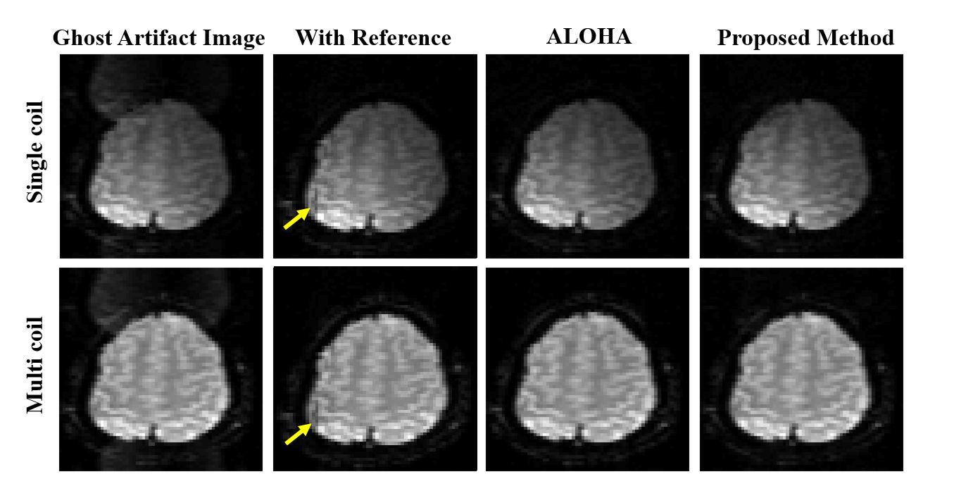
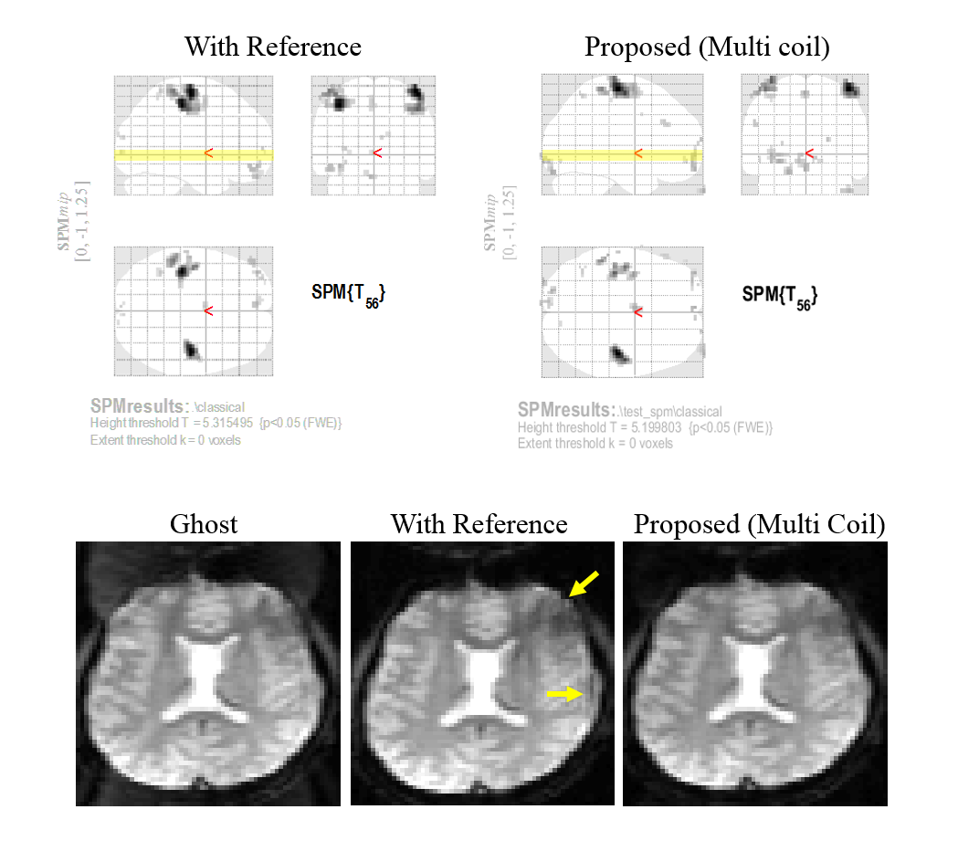
The reconstruction results are shown in Fig.3. The ghost artifact was removed by the proposed method, and it shows similar performance with ALOHA even for single-channel result without using multi-coil data. For the multi-channel data, all the 12 channel images are used for training and validation. As shown in Fig.4, the proposed method accurately located the left and right motor areas from the hand-squeezing experiment paradigm.

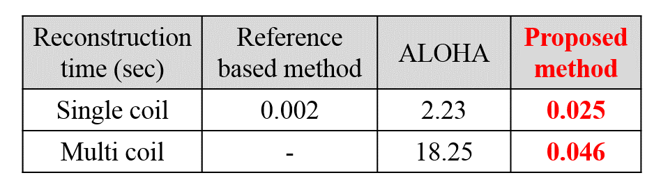
It took 2.5 hours to train the proposed network. For one-slice data reconstruction of single-channel and multi-channel data, it takes only 25ms and 46ms as shown in fig.5. Compared with ALOHA, the proposed method shows noticeable improvement in reconstruction time while showing good performance for ghost artifact removal.

Conclusion

Acknowledgements

References

1. Jin KH, Lee DW, Ye JC. A general framework for compressed sensing and parallel MRI using annihilating filter based low-rank Hankel matrix. IEEE Transactions on Computational Imaging. 2016; 2(4): 480-495.

2. Lee J, Jin KH, Ye JC. Reference‐free single‐pass EPI Nyquist ghost correction using annihilating filter‐based low rank Hankel matrix (ALOHA). Magn Reson Med. 2016; 76(6): 1775-1789.

3. Kang E, Min J, Ye JC. A deep convolutional neural network using directional wavelets for low-dose x-ray CT reconstruction. Medical Physics. 2017; 44(10).

4. Hammernik K., et al. Learning a variational model for compressed sensing MRI reconstruction. Proceedings of the International Society of Magnetic Resonance in Medicine(ISMRM). 2016; p.1088.

5. Wang S, et al. Accelerating magnetic resonance imaging via deep learning, IEEE International Symposium on in Biomedical Imaging (ISBI). 2016; p.514–517.

6. Ye JC, Han Y, Deep convolutional framelets: A general deep learning for inverse problems. arXiv preprint arXiv:1707.00372. 2017.