0554
Estimation of Pharmacokinetic Parameters in Dynamic Contrast Enhanced MRI via Random Forest Regression1Computer Science, Technical University of Munich, Munich, Germany, 2Neuroimaging Sciences, University of Edinburgh, Edinburgh, United Kingdom, 3Centre for Clinical Brain Sciences, University of Edinburgh, Edinburgh, United Kingdom, 4Institute for Digital Communication, University of Edinburgh, Edinburgh, United Kingdom, 5Cardiovascular Science, University of Sheffield, Sheffield, United Kingdom
Synopsis
We propose a novel alternative approach to estimate pharmacokinetic (PK) parameters of dynamic contrast enhanced (DCE)-MRI. Our approach leverages machine learning field and mainly targets to automatically learn temporal patterns of the voxel-wise concentration-time curves (CTCs) from a large amount of training samples in order to make accurate parameter estimations. We consider the estimation of parameters as a regression problem and specifically use Random Forest (RF) regression. We demonstrate its potential and utility to improve the conventional model-fitting based quantitative analysis of DCE-MRI especially in various noise conditions, and validate our method on clinical brain stroke datasets.
Introduction
The $$$T_1$$$-weighted dynamic contrast enhanced (DCE)-MRI is an imaging technique that provides a quantitative measure of pharmocokinetic (PK) parameters1, such as vascular permeability ($$$K^{\text{trans}}$$$) and fractional plasma volume ($$$v_p$$$). Tracer kinetic (TK) modeling2,3,4 is usually applied on the dynamic image series to estimate these physiological parameters which can be primarily used for diagnostic purpose in tumor5 and stroke6 studies. One of the key limitation of TK modeling methods is that they are simply based on the fitting of the voxel-wise PK parameters to contrast agent concentration-time curves (CTCs). However, the acquired voxel-wise CTCs are generally very noisy, hence the model fitting may likely produce substantial errors in PK parameter mapping7. In this work, we demonstrate a machine learning based approach to identify and learn the important features in temporal CTCs to directly output more robust estimates of PK parameters in DCE-MRI.Methods
Dataset: We perform experiments on fully-sampled DCE-MRI datasets acquired from three patients with clinically evident mild ischaemic stroke. DCE-MRI was acquired using a 1.5T clinical scanner with a 3D T1W spoiled gradient echo sequence (TR/TE = 8.24/3.1 ms, flip angle = 12$$$^{\circ}$$$, FOV = 24×24 cm, matrix = 256×192, slice thickness = 4 mm, 42 slices, 73 sec temporal resolution). The total acquisition time for DCE-MRI was approximately 24 minutes. Two pre-contrast acquisitions were carried out at flip angles of 2$$$^{\circ}$$$ and 12$$$^{\circ}$$$ to calculate longitudinal relaxation times ($$$T_{10}$$$).
Preprocessing: To generate noisy data, the noise-free (reference) data was corrupted by (1) undersampling the k-space, or (2) adding zero-mean Gaussian noise in the image space. Undersampling was retrospectively done in the $$$k_x-k_y$$$ plane using a randomized golden-angle sampling pattern8. Dynamic image intensities $$$S(\mathrm{r},t)$$$ were converted to contrast agent concentration $$$C(\mathrm{r},t)$$$ by the steady-state spoiled gradient echo (SGPR) signal equation9. The Parker's population-based arterial input function10 (AIF) was generated to obtain PK parameters using Patlak model3.
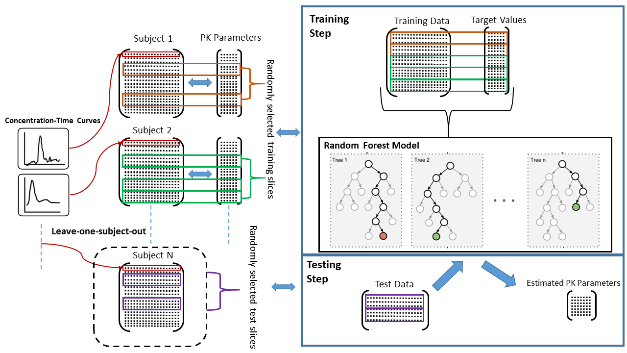
Random Forest Regression: The parameter estimation task is formulated as a regression problem which takes the voxel-wise $$$C(\mathrm{r},t)$$$ as input and generates the PK parameters ($$$K^{\text{trans}},v_p$$$) as output. In this work, we adopt the random forest (RF) regression that has been shown to be effective in a wide range of classification and regression problems11,12. We train a separate RF model to estimate each PK parameter. The overall regression task is defined as, $$\mathcal{M}(C(\mathrm{r}_i,t))=y_i;\quad i\in[1,N],\qquad(1)$$ where $$$y_i$$$ is the target parameter value for voxel $$$i$$$, $$$N$$$ is the total number of training samples (voxels), and $$$\mathcal{M}$$$ is the trained RF model. The target (reference) PK parameter values were estimated on noise-free data using Patlak model.
Training-Testing: Training and testing were carried out based on leave-one-patient-out cross-validation. The RF model $$$\mathcal{M}$$$ was trained with almost 340K voxels to learn important features from the input data to attain better parameter estimation. The pipeline of training-testing of RF model is provided in Figure 1.
Evaluation: The parameter estimates of our RF based method was compared with the estimations obtained from Patlak model in both noise-free and different noise conditions. The root-mean-square-error (RMSE) was used for quantitative evaluations of parameter estimation based on the following formula, $$RMSE=\sqrt{\frac{1}{N_i}\sum_{i=1}^{N_i} (y_i-f_i)^2},\qquad(2)$$ where $$$y_i$$$ is the target value, $$$f_i$$$ is the estimated value, and $$$N_i$$$ is the number of test samples.
Results and Discussion
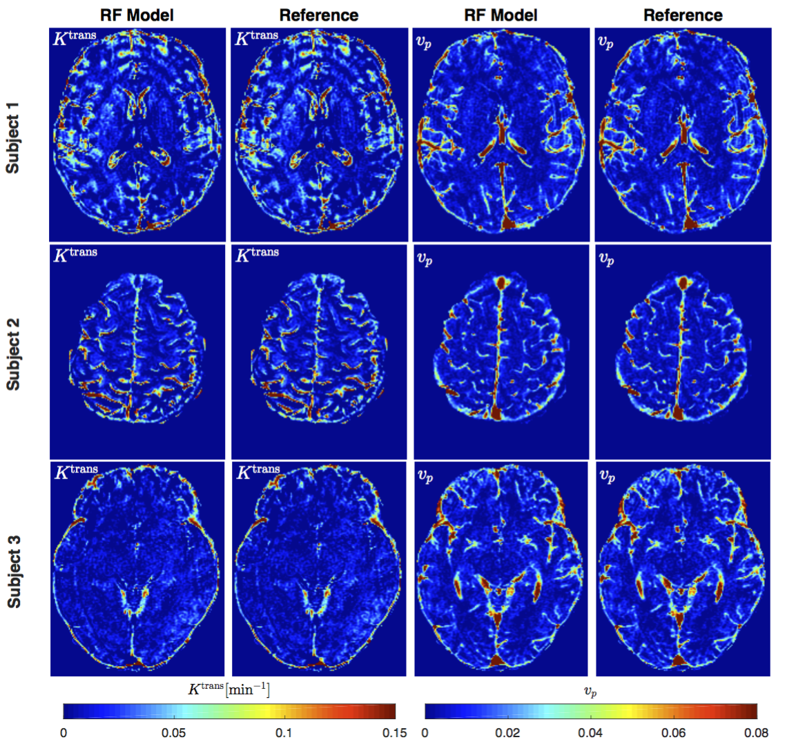
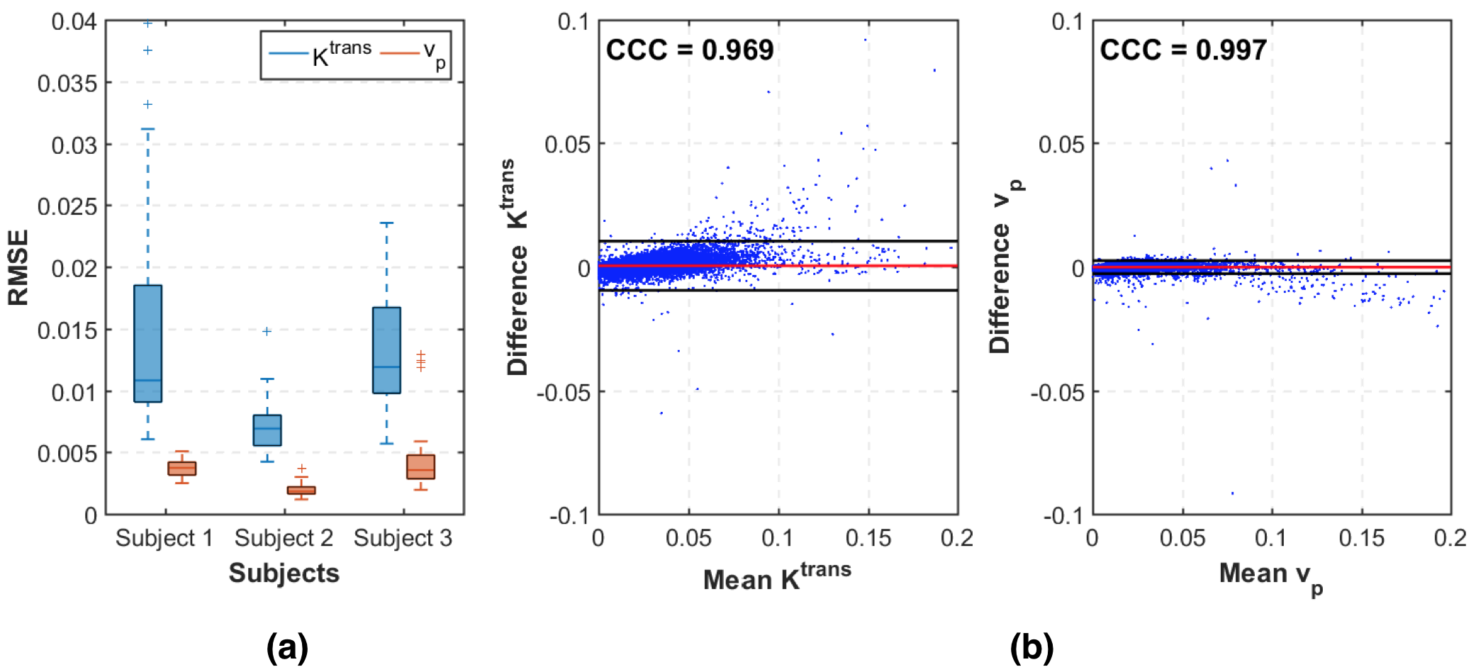
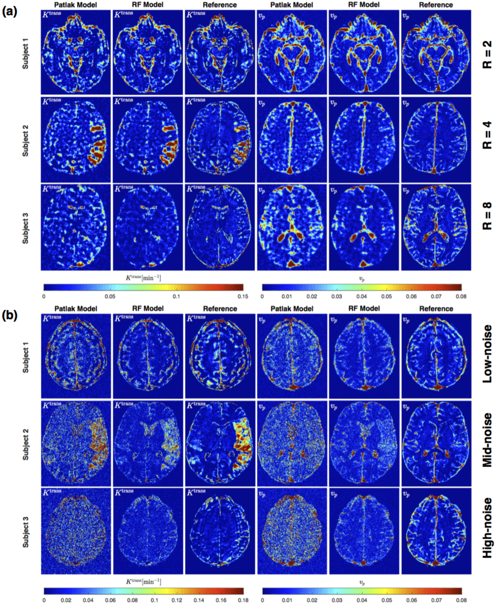
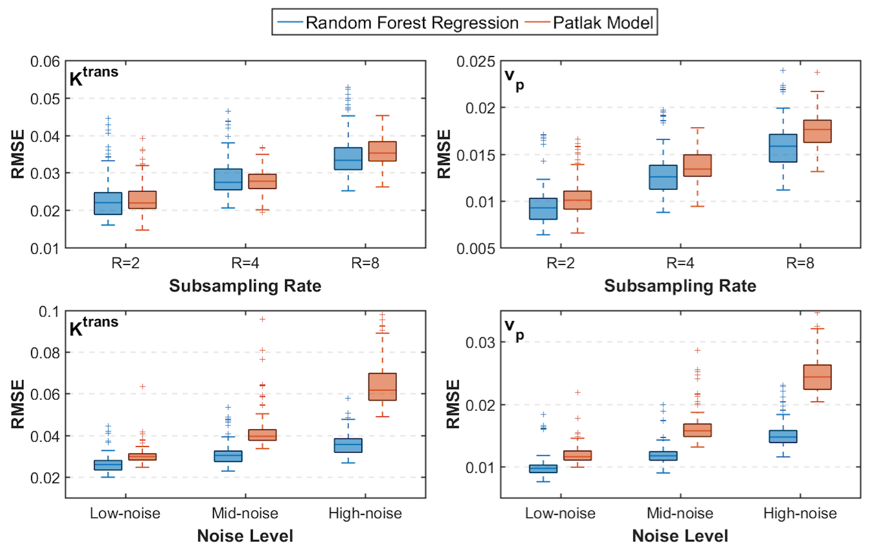
Figure 2 shows PK parameter maps estimated from noise-free data. The proposed RF model can yield parameter maps that are highly similar to reference. This is also evident in Bland-Altman plots as displayed in Figure 3. From the RMSE statistics in Figure 3, we can clearly observe that RF model provides more accurate estimation of $$$v_p$$$ than $$$K^{\text{trans}}$$$. Figure 4 depicts estimated PK maps in various noise conditions. The proposed RF model is able to mitigate the over-estimation of parameters that is observable in Patlak model and caused by high level of noise introduced into the data. Figure 5 quantitatively reveals that RF regression model achieves lower RMSE of PK parameters with respect to increasing noise levels, therefore it appears more robust to noise than Patlak model.Conclusion
We have demonstrated a new machine learning based approach to directly estimate PK parameters in DCE-MRI. This approach leverages large cohort of training data to learn significant characteristics and features of CTCs. Extensive experiments validated its efficacy in parameter estimation and robustness to various noise conditions. The proposed method is considerably faster than conventional model fitting. Training more than 300K samples takes around 5 minutes while testing takes only 1 second per slice. Future studies will aim at improving the estimation performance of RF model for high subsampling rates to potentially enable accelerated acquisitions of DCE-MRI, and testing our model on different tracer kinetic models such as extended Tofts model2 and two-compartment exchange model13.
Acknowledgements
The research leading to these results has received funding from the European Unions H2020 Framework Programme (H2020-MSCA-ITN- 2014) under grant agreement no 642685 MacSeNet. We also acknowledge Wellcome Trust (Grant 088134/Z/09/A) for recruitment and MRI scanning costs.References
1. Heye AK, Culling RD, del C. Valdes Hernandez M, Thrippleton MJ, Wardlaw JM. Assessment of blood-brain barrier disruption using dynamic contrast-enhanced MRI. a systematic review. NeuroImage. 2014;Clinical 6(Supplement C):262–274.
2. Tofts PS, Brix G, Buckley DL, et al. Estimating kinetic parameters from dynamic contrast-enhanced T1-weighted MRI of a diffusable tracer: Standardized quantities and symbols. Journal of Magnetic Resonance Imaging. 1999;10(3):223–232.
3. Patlak CS, Blasberg RG, Fenstermacher JD. Graphical evaluation of blood-to-brain transfer constants from multiple-time uptake data. Journal of Cerebral Blood Flow & Metabolism. 1983;3(1):1–7.
4. Sourbron SP, Buckley DL. Classic models for dynamic contrast-enhanced MRI. NMR in Biomedicine. 2013;26(8):1004–1027.
5. Türkbey B, Thomasson D, Pang Y, Bernardo M, Choyke PL. The role of dynamic contrast-enhanced MRI in cancer diagnosis and treatment. Diagnostic and Interventional Radiology. 2010;16:186–192.
6. Kassner A, Roberts TPL, Moran B, Silver FL, Mikulis DJ. Recombinant tissue plasminogen activator increases blood–brain barrier disruption in acute ischemic stroke: an MR imaging permeability study. American Journal of Neuroradiology. 2009;30:1864–1869.
7. Kelm BM, Menze BH, Nix O, Zechmann CM, Hamprecht FA. Estimating kinetic parameter maps from dynamic contrast-enhanced MRI using spatial prior knowledge. IEEE Transactions on Medical Imaging. 2009;28(10):1534–1547.
8. Zhu Y, Guo Y, Lingala SG, Lebel RM, Law M, Nayak KS. GOCART: GOlden-angle CArtesian randomized time-resolved 3D MRI. Magnetic Resonance Imaging. 2016;34(7):940–950.
9. Guo Y, Lingala SG, Zhu Y, Lebel RM, Nayak KS. Direct estimation of tracer-kinetic parameter maps from highly undersampled brain dynamic contrast enhanced MRI. Magnetic Resonance in Medicine. 2017;78(4):1566–1578.
10. Parker GJ, Roberts C, Macdonald A, Buonaccorsi GA, et al. Experimentally-derived functional form for a population-averaged high-temporal-resolution arterial input function for dynamic contrast-enhanced MRI. Magnetic Resonance in Medicine. 2006;56(5):993–1000.
11. Breiman L. Random forests. Machine Learning. 2001;45(1):5–32.
12. Criminisi A, Shotton J. Decision Forests for Computer Vision and Medical Image Analysis. Springer Publishing Company, Incorporated. 2013.
13. Nadav, G, Liberman G, Artzi M, Kiryati N, Bashat DB. Optimization of two-compartment-exchange-model analysis for dynamic contrast-enhanced MRI incorporating bolus arrival time. Journal of Magnetic Resonance Imaging. 2017;45(1):237–249.
Figures