0537
Calibrating variable flip angle (VFA)-based T1 maps: when and why a simple scaling factor is justified1CAMH, Toronto, ON, Canada
Synopsis
Variable Flip Angle (VFA)-based T1 maps are known to be prone to errors deriving from B1 errors (inaccurate knowledge of flip angles) and poor signal spoiling. In general, in vivo T1VFA values tend to overestimate T1 values obtained using a gold standard inversion recovery method :T1IR. Calibrating T1VFA with T1IR has been proposed but it requires knowledge of the exact relationship between these. This work models the contribution of B1 errors and poor spoiling to T1VFA errors and via simulations, the conditions for T1VFA/T1IR= constant (i.e. simple scaling) are derived. Experiments on phantoms and in vivo are used for validation.
Introduction
T1 brain maps, essential for probing brain microstructure, are difficult to produce accurately in vivo. Thus, a variety of T1 mapping methods are currently used1-9, leading to a lack of consensus of T1 values and a need to calibrate across methods7. A gold standard inversion recovery based T1 map (T1IR)8 is often used to validate and assess the accuracy of T1 maps. In particular, the variable-flip-angle (VFA) method, using a spoiled-gradient-echo (SPGR) sequence, has been shown to produce T1VFA that overestimate T1 values in vivo, relative to T1IR7. The main sources of T1VFA map errors are the errors in B1 maps (depicting the ratio of local to nominal α) and poor RF spoiling7,9-12. To correct for T1VFA errors, a calibration with respect to T1IR has been suggested although the exact form has not been given7. While it is tempting to use a simple scaling factor, this has not yet been justified, i.e., the conditions required for this have not been described. Thus, this constitutes the main goal of this work.Method
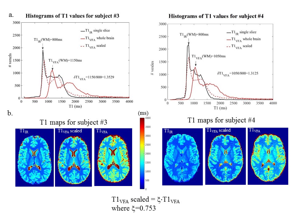
A simple scaling factor, ξ, can correctly calibrate a T1VFA map only if the relationship between T1VFA and T1IR is constant, or equally, the T1VFA error, δT1VFA, is constant: δT1VFA=T1VFA/T1IR =1/ξ. Here, a two-point VFA method is used to compute T1VFA from SPGR signals: S1(α1) and S2(α2) where Si=S0(1-E1)sin(B1·αi)/(1-E1cos(B1·αi)), for E1=exp(-TR/T1), B1=(αi)local/αi and S0=equilibrium signal. Simulations are used to model the effects of B1 errors and RF spoiling errors on T1VFA as follows.
Most B1 mapping methods produce approximately constant brain B1 error13-15: δB1=B1measured/B1true. Furthermore, the relationship δT1VFA vs δB1 is approximately independent of (B1,T1), over a range of relevant brain values (B1:0.8-1.3; T1:800-2000ms)4,16, but noise (low SNR) can compromise this16. Thus, given sufficient SNR, δB1 produces a constant brain δT1VFA and, in the absence of poor spoiling, a simple scaling factor: ξ=1/δT1VFA can be used to calibrate T1VFA maps.
Poor RF spoiling, resulting from poor RF seed, φ, selection or challenging parameters (e.g.,α>20°), can produce banding/ghosting artifacts and signal instabilities/bias12,17,18. Isochromat simulations have been used to propose φ values10,11,12,17,18, optimizing either signal accuracy or stability, but the models fail to predict the signal in vivo7,11. Thus, we take a different, novel approach. We assume that φ is chosen to obtain stable but biased signal with error: δS i=(Si)meas/Si. Using (α1,α2)=(3°,14°), we can assume δS1≈1 and simulate the effects of δS2 on δT1VFA .Using the SPGR signal equation, step-wise values of δS2=0.9:0.05:1.1 are used to compute T1VFA(S1,(S2)meas) and δT1VFA vs δB1 curves are traced out for relevant (B1,T1), at each step. The curves for δS2≠1 in Fig.1a show the simultaneous effect of δB1 and poor spoiling on δT1VFA. To a good approximation, these curves are independent of (B1,T1), as long as SNR is sufficient (Fig.1b). Thus, for a simple scaling factor to be justified, we propose the following conditions: SNR(S1)≥15, constant δB1, stable (S1,S2) with δS1=1 and constant δS2.
To test these conditions, experiments were performed at 3T (MR750, GE Healthcare) with a receive-only headcoil. A phantom (consisting of an aqueous MnCl2 solution in two beakers) and six volunteers were scanned in compliance with the institutional REB. (S1,S2) were acquired from full volume, 3D FSPGR sagittal scans: (1mm)3, ASSET=2, TR=10.7ms6. Repeat phantom measurements (3X) were obtained at several seed values around φ=50° (proposed for stability)11 and φ=115.4° (GE default). Three volunteers were also scanned thrice at φ=50° and 115.4°, and once at other φ values. Signal ratios across φ (i.e., normalizations) were used to test for biases. In vivo, B1MoS maps were produced using the Method of Slopes6 for T1VFA computations. Single slice, four-point T1IR were also produced8 per subject yielding ξ=T1IR/T1VFA , using white matter (WM) T1 values.
Results
Fig.2 shows repeated phantom measurement results. Data points represent average values over regions-of-interest (ROIs) shown in (a). CV =(STD/AVE)·100% maps show signal instabilities. Signal biases are tested using ratios/normalizations. Fig.3 shows in vivo results from signal stability and bias experiments at φ=50° and 115.4°. Fig.4 shows in vivo bias tests for other φ. ROIs are used to obtain signal instability/bias per φ, per tissue type. Fig.5 shows δT1VFA assessments in vivo.
Discussion and Conclusion
Phantom signal averaged in ROIs changes with φ>115.4° but remains temporally stable; poor spoiling causes local increased instability and nonuniform δS2 (shown in CV maps and normalized S2 images). In vivo S1 and S2 (for φ=50°) give stable signal with δS1=1 and constant whole brain δS2. Using these acquisitions and B1MoS, we demonstrated that the conditions for simple scaling were met, thus yielding consistent δT1VFA for all volunteers: AVE(δT1VFA)±STD(δT1VFA)=1.328±0.022, and ξ=1/AVE(δT1VFA)=0.753.Acknowledgements
No acknowledgement found.References
1. Warntjes JBM, Dahlqvist O, Lundberg P. Novel method for rapid, simultaneous T-1, T-2(*), and proton density quantification. Magnetic Resonance in Medicine 2007;57(3):528-537.
2. Freeman AJ, Gowland PA, Mansfield P. Optimization of the ultrafast Look-Locker echo-planar imaging T-1 mapping sequence. Magnetic Resonance Imaging 1998;16(7):765-772.
3. Deoni SCL. High-resolution T1 mapping of the brain at 3T with driven equilibrium single pulse observation of T1 with high-speed incorporation of RF field inhomogeneities (DESPOT1-HIFI). Journal of Magnetic Resonance Imaging 2007;26(4):1106-1111.
4. Cheng HLM, Wright GA. Rapid high-resolution T-1 mapping by variable flip angles: Accurate and precise measurements in the presence of radiofrequency field inhomogeneity. Magnetic Resonance in Medicine 2006;55(3):566-574.
5. Helms G, Dathe H, Dechent P. Quantitative FLASH MRI at 3T using a rational approximation of the Ernst equation. Magnetic Resonance in Medicine 2008;59(3):667-672.
6. Chavez S, Stanisz GJ. A novel method for simultaneous 3D B1 and T1 mapping: the method of slopes (MoS). Nmr in Biomedicine 2012;25(9).
7. Stikov N, Boudreau M, Levesque IR, Tardif CL, Barral JK, Pike GB. On the Accuracy of T-1 Mapping: Searching for Common Ground. Magnetic Resonance in Medicine 2015;73(2):514-522.
8. Barral JK, Gudmundson E, Stikov N, Etezadi-Amoli M, Stoica P, Nishimura DG. A Robust Methodology for In Vivo T-1 Mapping. Magnetic Resonance in Medicine 2010;64(4):1057-1067.
9. Hurley SA, Yarnykh VL, Johnson KM, Field AS, Alexander AL, Samsonov AA. Simultaneous variable flip angle-actual flip angle imaging method for improved accuracy and precision of three-dimensional T1 and B1 measurements. Magnetic Resonance in Medicine 2012;68(1):54-64.
10. Yarnykh VL. Optimal Radiofrequency and Gradient Spoiling for Improved Accuracy of T-1 and B-1 Measurements Using Fast Steady-State Techniques. Magnetic Resonance in Medicine 2010;63(6):1610-1626.
11. Preibisch C, Deichmann R. Influence of RF Spoiling on the Stability and Accuracy of T-1 Mapping Based on Spoiled FLASH With Varying Flip Angles. Magnetic Resonance in Medicine 2009;61(1):125-135.
12. Treier R, Steingoetter A, Fried M, Schwizer W, Boesiger P. Optimized and combined T-1 and B-1 mapping technique for fast and accurate T-1 quantification in contrast-enhanced abdominal MRI. Magnetic Resonance in Medicine 2007;57(3):568-576.
13. Morrell GR. A phase-sensitive method of flip angle mapping. Magnetic Resonance in Medicine 2008;60(4):889-894.
14. Pohmann R, Scheffler K. A theoretical and experimental comparison of different techniques for B1 mapping at very high fields. Nmr in Biomedicine 2013;26(3):265-275.
15. Lutti A, Hutton C, Finsterbusch J, Helms G, Weiskopf N. Optimization and Validation of Methods for Mapping of the Radiofrequency Transmit Field at 3T. Magnetic Resonance in Medicine 2010;64(1):229-238.
16. Chavez S. A simple method (eMoS) for T1 mapping is more accurate and robust than the Variable Flip Angle (VFA) method. ISMRM 23rd Annual Meeting and Exhibition. Toronto, Canada; 2015. p. 1673.
17. Epstein FH, Mugler JP, Brookeman JR. Spoiling of transverse magnetization in gradient-echo (GRE) imaging during the approach to steady state. Magnetic Resonance in Medicine 1996;35(2):237-245.
18. Zur Y, Wood ML, Neuringer LJ. SPOILING OF TRANSVERSE MAGNETIZATION IN STEADY-STATE SEQUENCES. Magnetic Resonance in Medicine 1991;21(2):251-263.
Figures
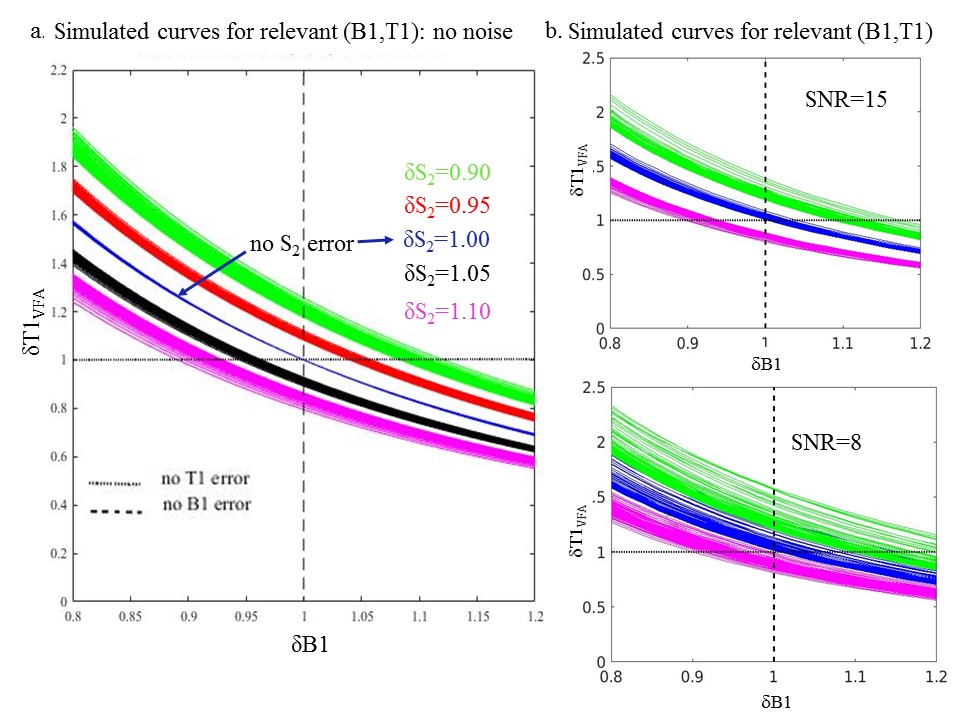
Fig.1 Simulated plots describing the relationships between δB1, δS2 and δT1VFA. (a) shows that for all relevant (B1,T1) values, the δT1VFA vs δB1 curves are still relatively consistent given a constant |δS2|>0 (small spread of same-coloured curves) so to a good approximation, we expect constant δT1VFA for constant values of δB1 and δS2. (b) shows the effect on the curves when Gaussian distributed noise with standard deviation=σ=S1/SNR, is added to S1 and S2. The independence of the curves on (B1,T1) values is compromised by noise as shown by the increased spread of equal-coloured curves for SNR=15 and 8.
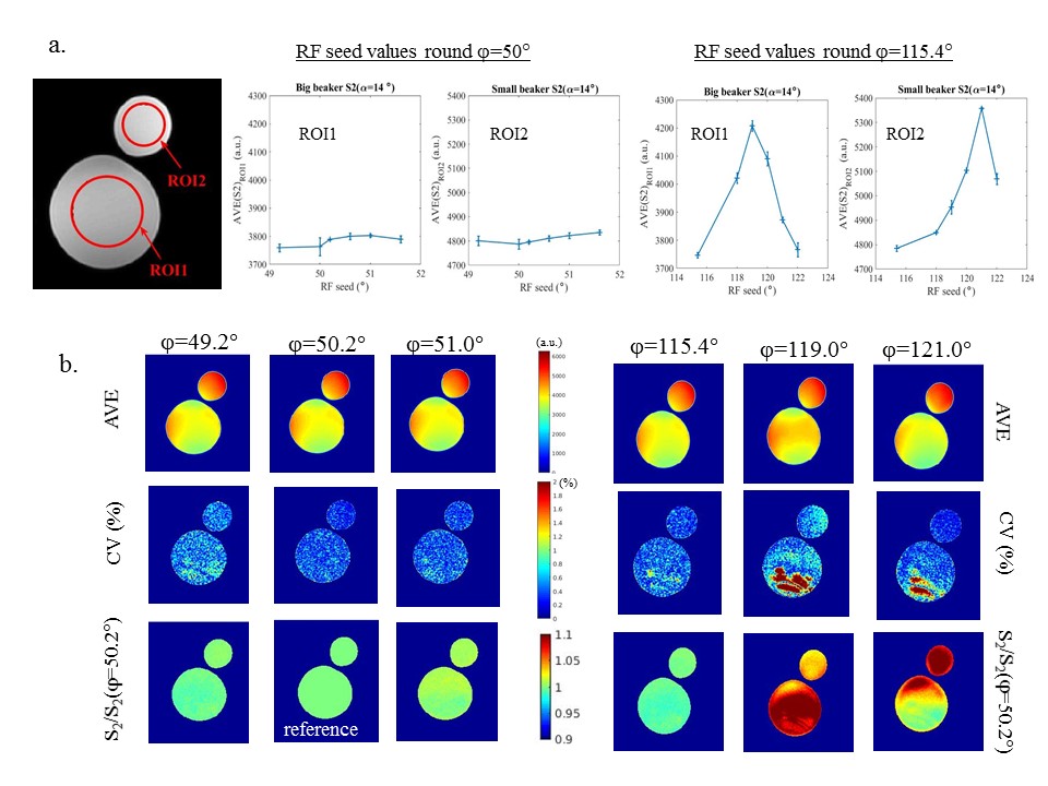
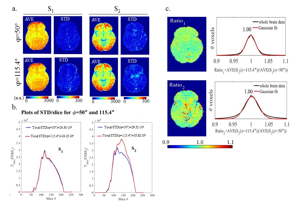
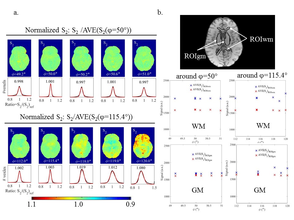
Fig.4 Results of signal bias measurements on one volunteer. (a) shows normalized S2 images for all φ. The images are single S2 measurements normalized by the temporal AVE(S2) obtained at either φ=50° (top) or φ=115.4°(bottom). Histograms of whole brain normalized S2 values (black lines) are shown with Gaussian fits (red) and peak values. Images for φtested < 118.0° look uniform. Histograms show constant whole brain δS2, to within experimental error, with small bias variations given by shifting peaks. (b) shows that for φtested < 118.0°, S1 and S2 are stable and consistent within structure. Results were similar for other volunteers.