Synopsis

A multislice method based on time-resolved imaging of contrast kinetics was developed for measurement of murine kidney size and function. A total of eight slices covering both kidneys were imaged with a temporal resolution of 1.23 sec/scan. The estimated kidney volume showed a good agreement with a three-dimensional volume scan. By fitting contrast kinetics using a modified bi-compartment model, renal perfusion and normalized glomerular filtration rate (GFR) were quantified, and subsequently used to calculate renal blood flow and GFR. In conclusion, this method allows simultaneous and reliable measurement of mouse kidney volume, perfusion, blood flow, and GFR.

Introduction

Methods

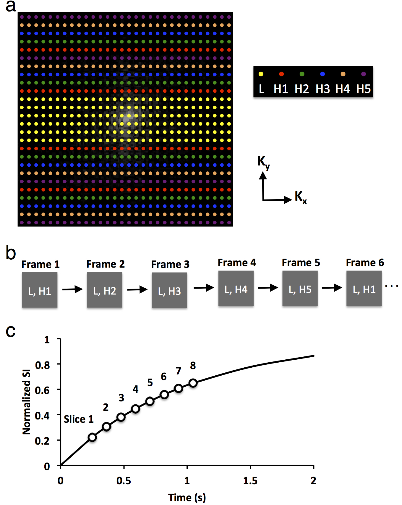
Imaging Method. Contrast dynamics were measured using the previously developed saturation recovery snapshot-fast low angle shot method². A TRICKS-based k-space data acquisition scheme was developed to facilitate multislice imaging (Fig. 1). The k-space was segmented into low (L, 28 center lines) and high (H, 100 peripheral lines) frequency lines in phase encoding direction (Fig. 1a). The H lines were further divided into five groups, as noted in different colors. During data acquisition, while the L lines were constantly sampled, only one of the H groups was acquired (Fig. 1b). An acceleration factor of 2.7 was achieved by this acquisition scheme, allowing imaging of eight axial slices at a temporal resolution of 1.23sec/scan. The eight slices were sampled at saturation recovery delays from 0.25 to 1.05sec (Fig. 1c).

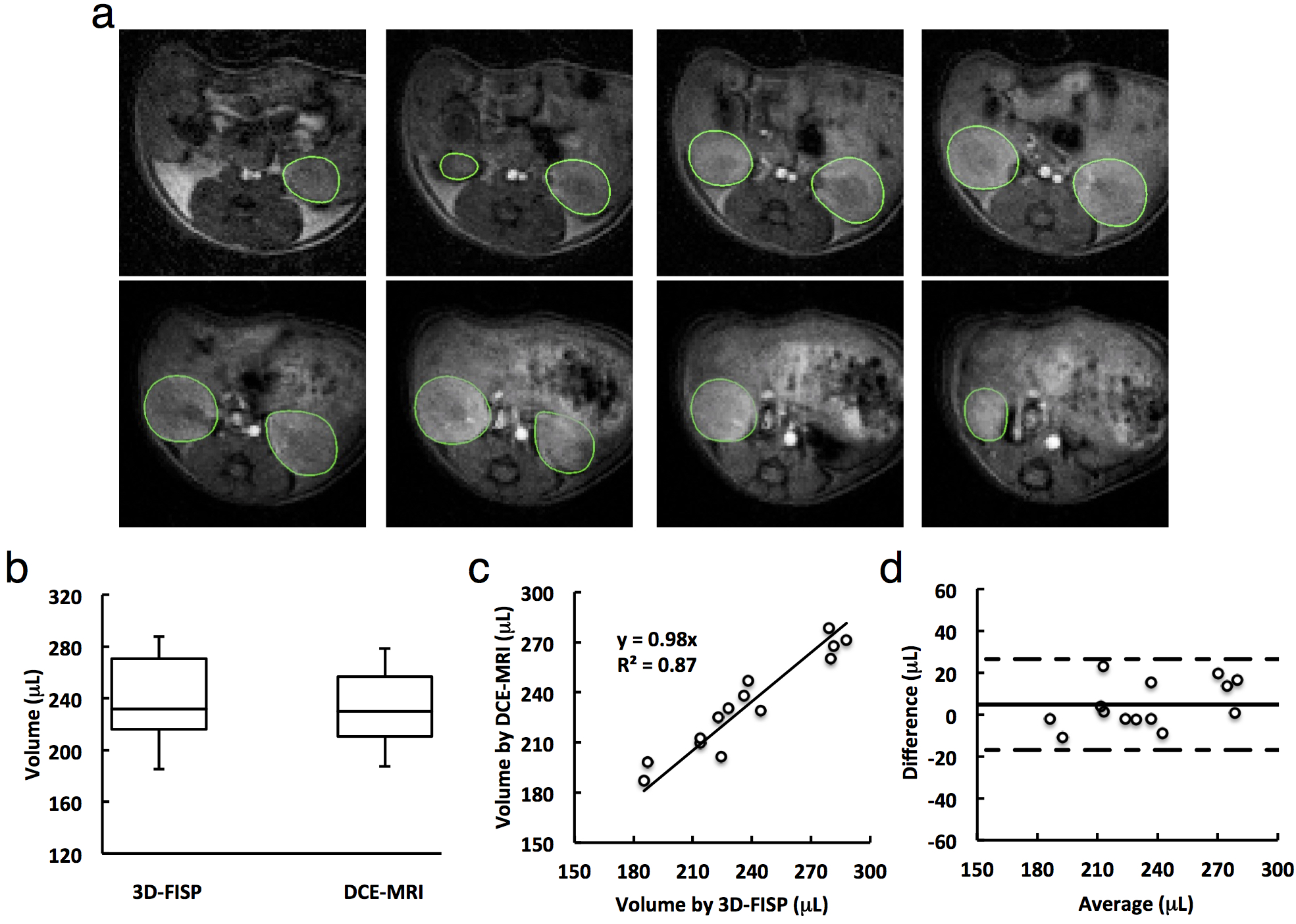
Animal Study. MRI studies were performed on a vertical 16.4 T scanner (Bruker, Billerica, MA) equipped with a 38-mm inner diameter birdcage coil. Seven 3-month-old male C57/BL6 mice were used. A homemade catheter with a fine needle (30G) was placed and secured in the tail-vein for injection of contrast agent. For each slice, ten proton density (M₀) images were acquired with a repetition time of 18 sec. Following the acquisition of ten baseline T₁-weighted (M_t) images, 20 mL of 37.5mM gadodiamide was injected through the tail-vein within 2s, after which the M_t images were acquired repetitively. Other imaging parameters were: encoding scheme, central; TR 17.9ms; TE 0.8ms; flip angle 15°; slice thickness 1.5mm; FOV 3.0×3.0cm²; matrix size 128×128; number of repetitions 100. T₁ was estimated by a two-point mono-exponential fitting and the change in R₁ (ΔR₁) from baseline was used as an index of Gd concentration. A three-dimensional fast imaging with steady precession (3D-FISP) sequence was also used to measure kidney volume using the following parameters: TR 14ms; TE 2.7ms; flip-angle 20°; FOV 5.12×2.56×1.28cm³; matrix size 256×128×64; number of averages 2.

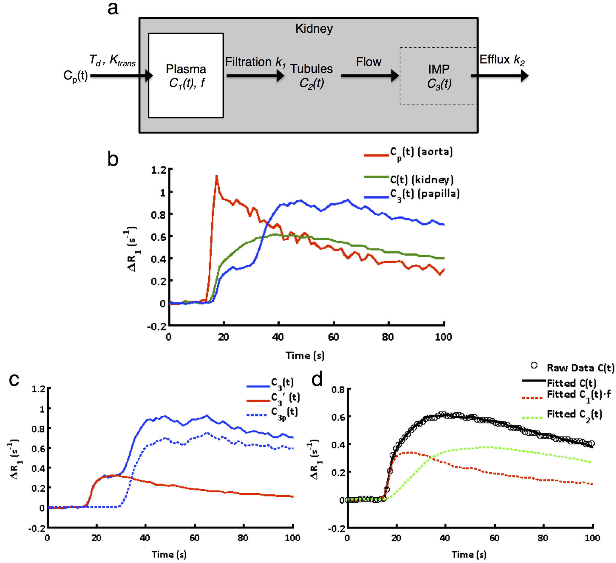
Image Analysis. Renal volumes (V) were measured from the 3D-FISP images by manual segmentation. For DCE-MRI image reconstruction, view sharing of adjacent scans was used. Kidney volume is measured from images at early (vascular) phases of contrast enhancement by manual segmentation. The measured contrast kinetics were fitted using a previously developed bi-compartmental model, which was modified by adding a transit delay (T_d) of blood from abdominal aorta to kidney (Fig. 2a). Changes in C₁(t) and C₂(t) can be described by the kinetic equations:

$$\frac{\text{d}C_{1}(t)}{\text{d}t}=K_{trans}(C_{p}(t-T_{d})-C_{1}(t))$$

$$\frac{\text{d}C_{2}(t)}{\text{d}t}=k_{1}C_{1}(t)-k_{2}C_{3}^{'}(t)$$

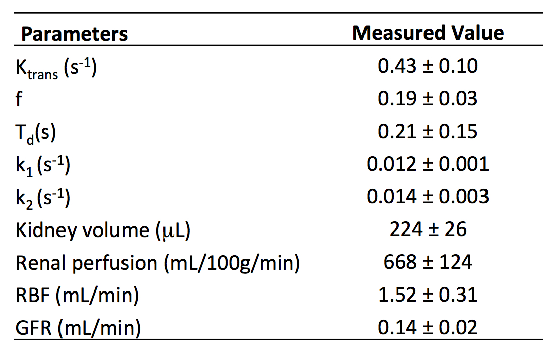
where C₃(t) is decomposed into perfusion (C_3p(t)) and tubular transit (C₃^’(t)). Total gadolinium concentration in the kidney is C(t)=C₁(t)×f+C₂(t). The five unknown parameters: K_trans, T_d, f, k₁ and k₂ were fitted with the least-squares algorithm. Then GFR was calculated as k₁×V×60, renal perfusion as K_trans×f×60×100/(1-Hct), and renal blood flow as perfusion×V.

Results

The representative whole-kidney Gd dynamics in aorta, kidney parenchyma, and inner medulla papilla (IMP) are shown in Fig. 2b. The decomposition of IMP gadolinium concentration (C₃(t)) into the perfusion (C_3p(t)) and filtration (C₃^’(t)) components is shown in Fig. 2c. The representative raw and model-fitted gadolinium dynamics in the renal parenchyma as well as the vascular (C₁(t).f) and tubular (C₂(t)) compartments are shown in Fig. 2d. Representative manually-traced kidney contours on the M_t images are shown in Fig. 3a. The estimated kidney volume from DCE-MRI showed a good agreement with that from the 3D volume scan (Fig. 3b-d). Fig. 4 shows the measured kidney parameters, which agree well with the previously measured values².

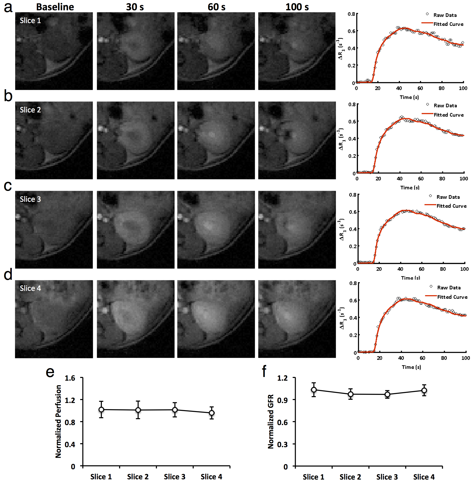
We also took the opportunity to compare renal perfusion and GFR at different slices of the kidney. Representative M_t images from four slices of the same kidney at baseline and 30, 60, and 100 sec post-contrast, along with the model fitting of their respective contrast kinetics, are shown in Fig. 5a-d. The measured renal perfusion (Fig. 5e) and GFR (Fig. 5f) from different slices showed minimal variation.

Conclusion

Acknowledgements

References

1. Annet L, Hermoye L, Peeters F, Jamar F, Dehoux JP, Van Beers BE. Glomerular filtration rate: assessment with dynamic contrast-enhanced MRI and a cortical-compartment model in the rabbit kidney. J Magn Reson Imaging 2004;20:843-849.

2. Jiang K, Tang H, Mishra PK, Macura SI, Lerman LO. Measurement of Murine Single-Kidney Glomerular Filtration Rate Using Dynamic Contrast-Enhanced MRI. Magn Reson Med 2017.

3. Korosec FR, Frayne R, Grist TM, Mistretta CA. Time-resolved contrast-enhanced 3D MR angiography. Magn Reson Med 1996;36:345-351.