Synopsis

Advanced diffusion imaging of the spinal cord is hampered by low signal-to-noise ratio, leading to strong Rician bias in magnitude images. Here, we investigate how to mitigate such bias studying complex-valued 3T diffusion scans of the cervical cord. We test two approaches, based on decorrelated phase (DP) and total variation (TV) filtering, corroborating results with simulations. The DP and TV methods, proposed for the brain, can be applied successfully also in the cord. Moreover, they appear useful pre-processing tools for image denoising, as state-of-the-art noise removal based on Marčenko-Pastur principal component analysis (MP-PCA) performs better on complex-valued as opposed to magnitude data.

Introduction

Precision and accuracy of diffusion MRI (dMRI) signal analyses are respectively compromised by noise fluctuations and noise-floor bias¹ in low signal-to-noise ratio (SNR) regimes². While rephasing complex-valued images has been proposed as a way to mitigate noise-floor bias^1,3, so far dMRI data are still commonly stored as magnitude images due to random phase variations across shots. Denoising alorithms to increase precision^4,5 are still typically applied on magnitude data.

Here we combine rephasing of complex-valued data with promising Marčenko-Pastur (MP) principal component analysis (PCA) denoising^6,7. MP-PCA relies on the redundancy of acquisitions, whereby the number of measurements greatly exceeds the number of signal sources. Using complex-valued data doubles the measurements, but random phase patterns⁸ may overall reduce the redundancy and decrease MP-PCA performance. We analyse in vivo and synthetic data to identify optimal strategies for rephasing spinal cord dMRI, assessing their benefit for MP-PCA, with a goal to achieve maximal noise removal, free from noise-floor bias.

Methods

Imaging

Four healthy volunteers (2 males; age 28-40) were scanned on a 3T Philips Achieva system, acquiring axial-oblique anatomical and diffusion-weighted (DW) images (5 b=0; {4, 10, 18, 28} gradient directions at b = {300, 1000, 2000, 2800} s/mm²; δ/Δ of 20/33 ms; cardiac-gated ZOOM-EPI⁹; delay: 150 ms; TE/TR: 71ms/12 heart beats; resolution: 1×1 mm²; matrix size: 64×48; 12 slices, 5 mm-thick; half scan factor: 0.6). Reconstructed images were obtained as complex-valued following CLEAR-based coil combination¹⁰.

Rephasing

Complex-valued images were rephased to map the signal intensity onto the real part with custom implementations of total variation¹ (TV) and decorrelated phase³ (DP) filtering algorithms, whose best settings (DP kernel; TV weight) were found by optimising within the cord (segmented with SCT^11,12) the ratio between imaginary root-mean-square (RMS) amplitude and noise standard deviation σ (RMS/σ=1 for ideal rephasing). Standard diffusion tensor (DT) metrics were obtained from magnitude and rephased real images.

Denoising

We synthesised a realistic complex-valued DW scan, generating noise-free signal intensity according to the DT model and realistic background phase via slice-wise median filtering of cos(φ/2) (φ: phase measurements in the subject with least motion). We used tissue-dependent DT¹³ and relaxation^14,15 parameters, with voxel-wise tissue fractions from SCT template/atlas, non-linearly warped¹¹ to the subject, introducing within-tissue variability.

We corrupted real/imaginary parts of the signal with Gaussian noise and performed slice-by-slice denoising to estimate the underlying signal in five ways:

1. denoising of magnitude followed by Rician bias mitigation¹⁶;
2. denoising of real part after rephasing;
3. independent denoising of real/imaginary parts;
4. denoising of complex-valued data;
5. denoising of real/imaginary part concatenation.

We tested 3-5 also after rephasing, quantifying denoising accuracy/precision as median and inter-quartile range (IQR) of percentage relative errors. Denoising strategies 1-5 were also tested in vivo.

Results

Rephasing

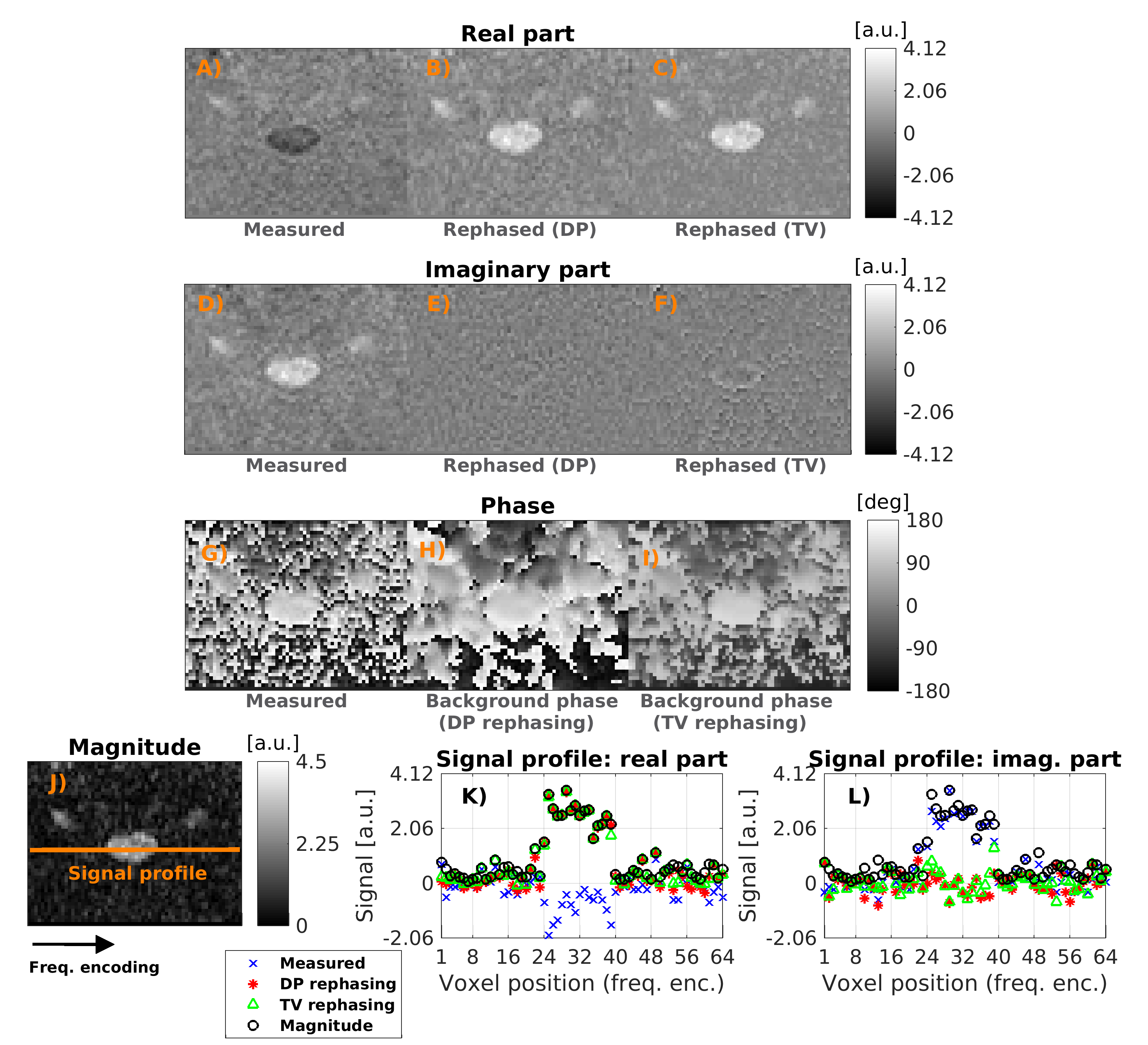
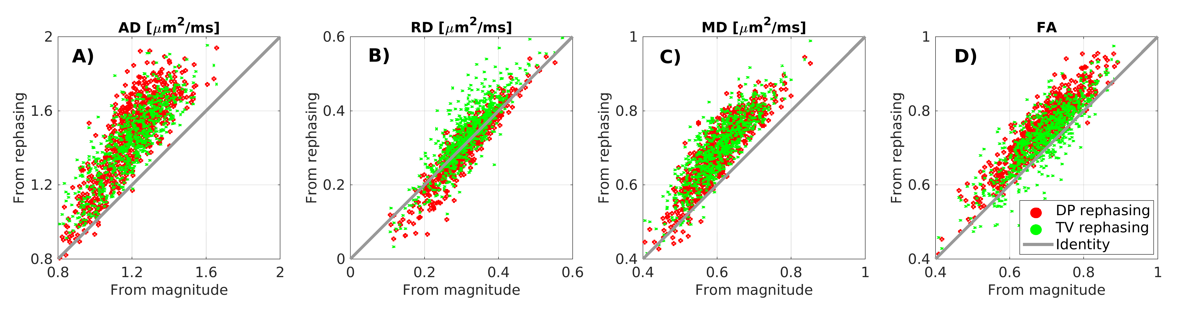
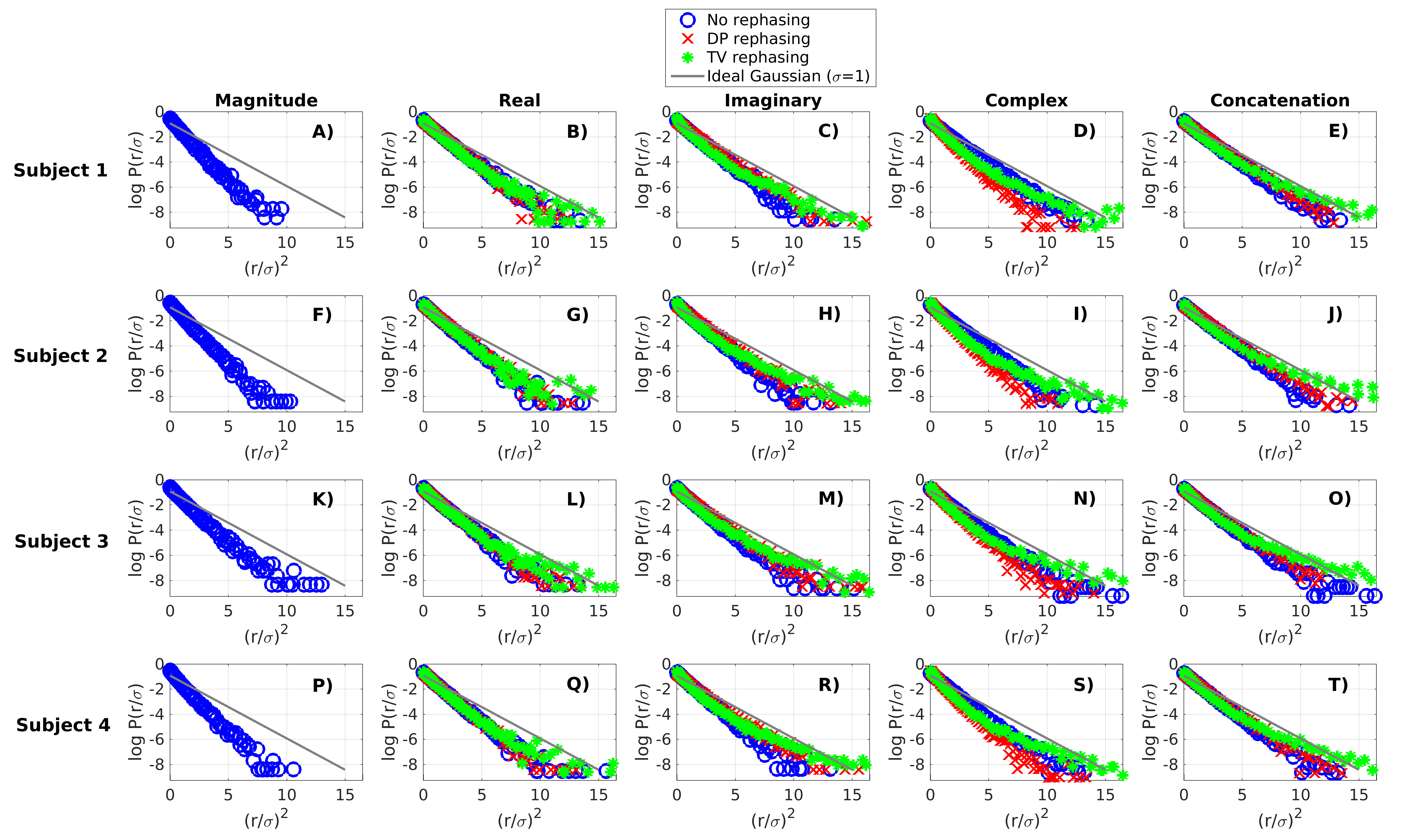
Optimal rephasing (RMS/σ≈1) is obtained in vivo using G3F1/G3F1H kernels³ for DP (non-DW/DW) and regularisation weight 4/0.75 (non-DW/DW) for TV filtering. Rephasing reduces the signal in the imaginary part and preserves Gaussian noise statistics in the real part, avoiding Rician bias (figure 1). Bias-free rephased signals lead to higher values of diffusivity and fractional anisotropy (figure 2). The strongest differences are seen for axial diffusivity: the larger the diffusivity, the closer DW signals get to noise floor.

Denoising

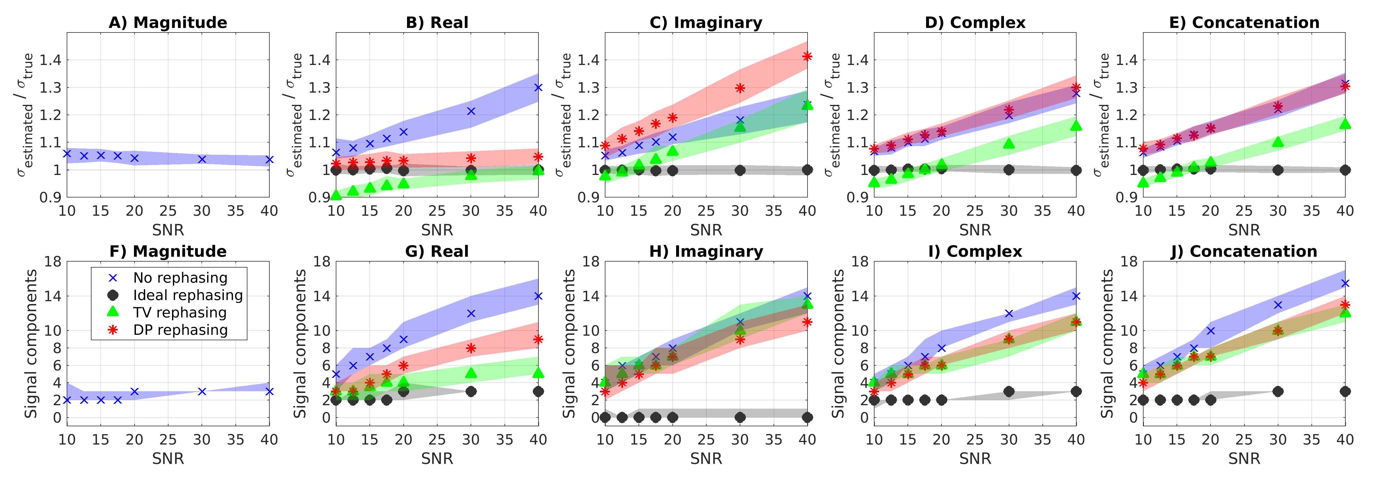
Figure 3 shows estimated noise level and information-carrying (“significant”) signal’s principal components from simulations. DP-based rephasing gives more accurate estimates of the noise level on complex-valued data, similar to those from magnitude denoising, although slight overestimations is seen at high SNR. Rephasing mitigates random phase fluctuations thereby reducing the number of signal components in the real channel, thereby improving MP-PCA performance.

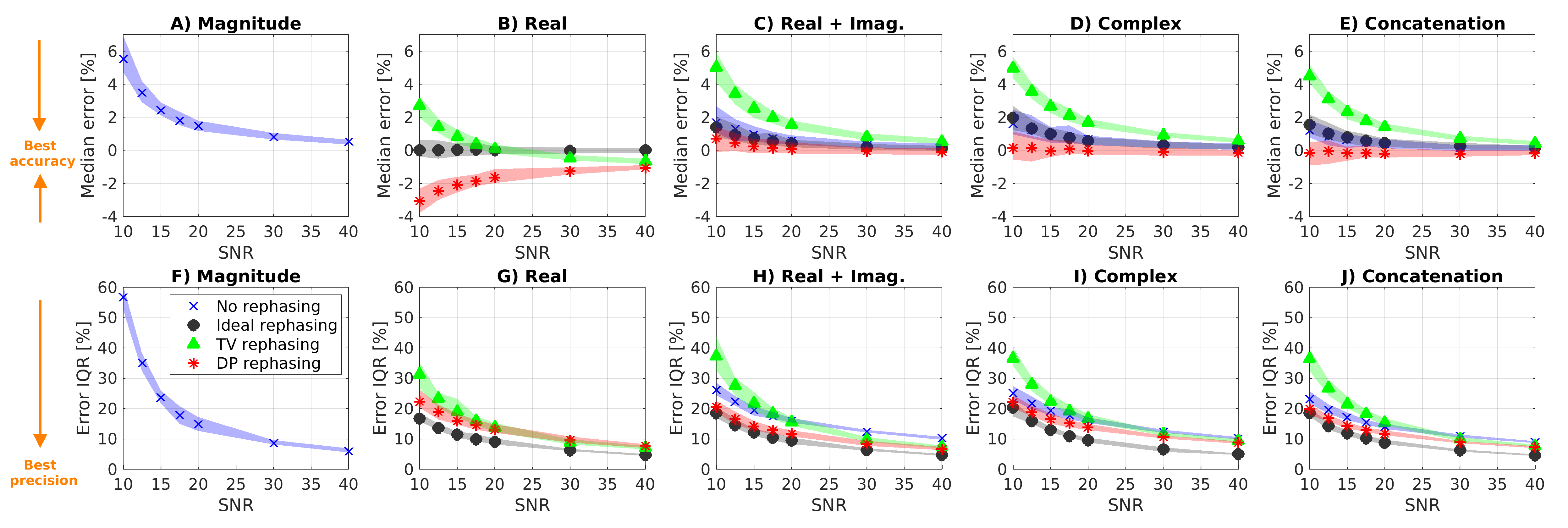
Figure 4 shows accuracy/precision of denoising in simulations. Denoising complex-valued data provides better accuracy/precision than denoising the magnitude. The best denoising is obtained after rephasing, and when residual signal left in the rephased imaginary channel is combined with the real part.

Figure 5 shows residuals (denoising output minus input) in vivo. Accounting for the complex-valued nature of the data provides better performances than denoising the magnitude: residuals are Gaussian over ~3σ, ensuring removal of noise but not anatomy^6,7. The best denoising is obtained on the concatenation of real/imaginary parts after rephasing, which doubles the number of measurements.

Discussion

Conclusions

Acknowledgements

References

1. Eichner C, Cauley SF, Cohen-Adad J, et al. Real diffusion-weighted MRI enabling true signal averaging and increased diffusion contrast. NeuroImage 2015; 122: 373-384.

2. Gudbjartsson H and Patz S. The Rician distribution of noisy MRI data. Magn Reson Med 1195; 34(6): 910-914.

3. Sprenger T, Sperl JI, Fernandez B, et al. Real valued diffusion-weighted imaging using decorrelated phase filtering. Magn Reson Med 2017; 77(2): 559-570.

4. Manjón JV, Coupé P, Martí-Bonmatí L, et al. Adaptive non-local means denoising of MR images with spatially varying noise levels. J Magn Reson Imaging 2010; 31(1): 192-203.

5. Knoll F, Bredis K, Pock T, et al. Second order total generalized variation (TGV) for MRI. Magn Reson Med 2011; 65(2): 480-491.

6. Veraart J, Fieremans E and Novikov DS. Diffusion MRI noise mapping using random matrix theory. Magn Reson Med 2016; 76(5): 1582-1593.

7. Veraart J, Novikov DS, Christiaens D et al. Denoising of diffusion MRI using random matrix theory. NeuroImage 2016; 142: 394-406.

8. Verma T and Cohen-Adad J. Effect of respiration on the B0 field in the human spinal cord at 3T. Magn Reson Med 2014; 72(6): 1629-1636.

9. Wheeler-Kingshott CA, Parker GJ, Symms MR, et al. ADC mapping of the human optic nerve: increased resolution, coverage, and reliability with CSF-supressed ZOOM-EPI. Magn Reson Med 2002; 47(1): 24-31.

10. Wallner BK, Edelman RR, Bajakian RL, et al. Signal normalisation in surface-coil MR imaging. Am J Neuroradiol 1990; 11(6): 1271-1272.

11. De Leener B, Lévy S, Dupont SM, et al. SCT: Spinal Cord Toolbox, an open-source software for processing spinal cord MRI data. NeuroImage 2017; 145(Pt A): 24-43.

12. De Leener B, Kadoury S, Cohen-Adad J. Robust, accurate and fast automatic segmentation of the spinal cord. NeuroImage 2014; 98: 528-536.

13. Grussu F, Schneider T, Zhang H et al. Neurite orientation dispersion and density imaging of the healthy cervical spinal cord in vivo. NeuroImage 2015; 590-601.

14. Smith SA, Edden RA, Farrell JA, et al. Measurement of T1 and T2 in the cervical spinal cord at 3 Tesla. Magn Reson Med 2008; 60(1): 213-219.

15. Volz S, Nöth U, Jurcoane A, et al. Quantitative proton density mapping: correcting the receiver sensitivity bias via pseudo proton densities. NeuroImage 2012; 63(1): 540-552.

16. Koay CG and Basser PJ. Analytically exact correction scheme for signal extraction from noisy magnitude MR signals. J Magn Reson 2006; 179(2): 317-322.