Synopsis

The primary focus of this work is to introduce a novel deep learning framework, which synergistically combines the benefits of model-based image recovery with the power of deep learning. This work enables the easy exploitation of prior information available from calibration scans, in addition to significantly reducing the number of network parameters, amount of training data required, and computational complexity. More importantly, the insensitivity of the learned model to the acquisition parameters also facilitates its easy reuse with a range of acquisition settings.

Introduction

Current deep learning based image recovery frameworks often rely on large networks to invert the k-space data, which requires considerable training data and computational power. Also, they cannot readily exploit prior information that is often available from calibration data or other sources, besides being heavily dependent on the specific acquisition parameters. The primary focus of this work is to synergistically combine the power of deep learning with the classical model-based reconstruction framework. We systematically integrate a residual learning convolutional neural network (CNN) as a plug-and-play prior, with the following benefits:

• Ability to be combined with other priors (e.g., field map, coil sensitivities, navigator information): The main difference of the unrolled CNN with the one in [3] is the use of the same shared weights at each iteration. In addition to reducing the number of network parameters, this also makes the recursive structure consistent with a model-based framework, which facilitates the easy combination with other priors.
• The universality of the learned model: A single learned model can recover image data acquired with different undersampling factors and acquisition settings.
• Fewer trainable parameters: This reduces the demand for training data and enables faster training. We demonstrate the utility of the proposed framework in recovering parallel MRI data from multi-coil datasets.
• Ability to exploit the power of software platforms such as Tensorflow, as opposed to variational deep learning methods such as [5].
  

Method

We formulate the reconstruction of parallel MRI data as the following optimization problem that incorporates deep CNN and coil information as priors.

\begin{equation} \nonumber \arg \min_{x_i} \sum_{i=1}^M\left( \underbrace{ \|\mathbf A\,\mathbf x_i-\mathbf b_i\|_2^2} _{\mbox{data consistency}} + \underbrace{{\lambda_1}~\|\mathbf x_i-\mathcal D_{\mathbf w}(\mathbf x_i)\|^2 } _{ \mbox{CNN-based denoiser} } \; + \underbrace{\lambda_2 \|\mathbf x_i - \mathcal P_{\mathcal C}(\mathbf x_i)\|^2 } _{\mbox{coil information}} \right)\end{equation}

Here, $$$\mathbf A = \mathbf S\mathbf F$$$, where $$$\mathbf S$$$ is the sampling operator, and $$$\mathbf F$$$ is the Fourier transform. $$$\mathcal N_{\rm w}(x)=\mathbf x-\mathcal D_{\rm w}(\mathbf x)$$$ is a learned CNN estimator of noise and alias patterns, which depends on the learned parameters $$$\mathbf w$$$. We assume that the data is acquired using $$$M$$$ coils, whose coil sensitivities are specified by $$$c_i\; i=1,\dots,M$$$. We consider the joint recovery of $$$\mathbf x_i\; i=1,\dots,M$$$ from the undersampled measurements $$$\mathbf b_i = \mathbf A\mathbf x_i$$$. We observe that the different coil sensitivity weighted images are restricted to a constraint space $$$ \mathcal C: ~~\mathbf x_i = \mathbf c_i \cdot \mathbf x;~\forall i=1,\dots,M $$$ where the $$$\cdot$$$ operation indicates element-wise multiplication of the vectors and $$$\mathbf x$$$ is the coil combined image to be reconstructed. We minimize the cost function by alternating between the following steps for all $$$i=1,\dots,M.$$$

\begin{eqnarray}\nonumber \mathbf z_i[n] &=& \mathcal D_{\mathbf w}\left(\mathbf x_i[n]\right),\\\nonumber \mathbf y_i[n] &=& \mathcal P_{\mathcal C}\left(\mathbf x_i[n]\right) = \frac{\mathbf c_i[n]^* \cdot \mathbf x_i[n]}{\sum_{i=1}^M \left|\mathbf c_i[n]\right|^2} ,\\\nonumber \mathbf x_i[n+1] &=&\left(\mathbf A^H\mathbf A + (\lambda_1 +\lambda_2) \;\mathbf I\right)^{-1} \left(\mathbf A^H \mathbf b_i + \lambda_1~ \mathbf z_i[n]+ \lambda_2 \mathbf y_i[n] \right)\end{eqnarray}

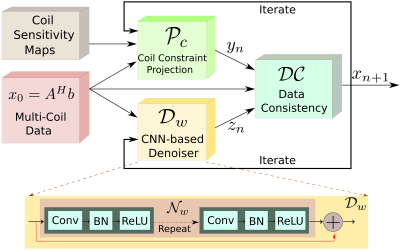
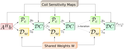
The regularization parameters $$$\lambda_1$$$ and $$$\lambda_2$$$ are set as trainable. We note that the same network weights are re-used at the channels and all the iterations. The outline of the iterative framework is shown in Fig. 1 whereas the unrolled network displayed in Fig. 2.

Experiments and Results

For validation, MRI data were acquired using a 3D T2 CUBE sequence with a matrix size of $$$256 \times 256 \times 208$$$ using a 16-channel array. We retrospectively undersampled the phase encodes to train and test the framework. Out of the 208 slices, we selected 90 slices that had reliable information for training. Dimensionality reduction using Principal component analysis (PCA) was applied to reduce the number of channels from 16 to 4. The coil sensitivity maps were estimated from the central k-space regions of each slice. A total of 360 slices from four subjects were used for training whereas 90 slices from the fifth subject were used during testing.

We used a five-layer model with 64 filters at each layer to implement $$$\mathcal N_w$$$. Each layer consists of convolution (conv) followed by batch normalization (BN) and a non-linear activation function ReLU. The proposed iterative model was unrolled assuming ten iterations and implemented in TensorFlow. At each 2D convolution, 64 filters of size $$$3\times 3$$$ were learned. The analytical form of the data consistency (DC) update enabled us to implement it as a separate layer, which facilitated the evaluation of the analytical gradients for backpropagation.

Conclusions

Acknowledgements

References

[1]. Shiqian Ma, Wotao Yin, Yin Zhang, and Amit Chakraborty, “An Efficient Algorithm for Compressed MR Imaging using Total Variation and Wavelets,” in Computer Vision and Pattern Recognition, 2008, pp. 1–8.

[2]. Stanley H. Chan, Xiran Wang, and Omar A. Elgendy, “Plug-and-Play ADMM for Image Restoration: Fixed Point Convergence and Applications,” IEEE Transactions on Computational Imaging, vol. 3, no. 1, pp. 84–98, 2017.

[3]. Jo Schlemper, Jose Caballero, Joseph V. Hajnal, Anthony Price, and Daniel Rueckert, “A Deep Cascade of Convolutional Neural Networks for MR Image Reconstruction,” in Information Processing in Medical Imaging, 2017, pp. 647–658.

[4]. Steven Diamond, Vincent Sitzmann, Felix Heide, and Gordon Wetzstein, “Unrolled Optimization with Deep Priors,” in arXiv:1705.08041, 2017, pp. 1–11.

[5]. Kerstin Hammernik, Teresa Klatzer, Erich Kobler, Michael P. Recht, Daniel K Sodickson, Thomas Pock, and Florian Knoll,“Learning a Variational Network for Reconstruction of Accelerated MRI Data,” in arXiv:1704.00447v1., 2017, pp. 1–29.

[6]. Sajan Goud Lingala, Yue Hu, Edward DiBella, and Mathews Jacob, “Accelerated dynamic MRI exploiting sparsity and low- rank structure: kt SLR,” IEEE Transactions on Medical Imaging, vol. 30, no. 5, pp. 1042–1054, 2011.