0437
Dynamic Causal Modelling with neuron firing model in Generalized Recurrent Neural Network framework1Department of Electrical and Computer Engineering, New York University, Brooklyn, NY, United States, 2Department of Radiology, New York University, New York, NY, United States
Synopsis
DCM-RNN is a Generalized Recurrent Neural Network accommodating the Dynamic Causal Modelling (DCM), which links the biophysical interpretability of DCM and the power of neural networks. It significantly extends the flexibility of DCM, provides unique parameter estimation methods, and offers neural network compatibility. In this abstract, we show how to incorporate neuron firing model into DCM-RNN with ease. An effective connectivity estimation experiment with simulated fMRI data shows that the influence of the firing model is substantial. Ignoring it, as the classical DCM does, can lead to degraded results.
Introduction
Dynamic Causal Modelling (DCM)1 is a highly nonlinear generative model used to infer the causal architecture in the brain from biophysical measurements, such as functional magnetic resonance imaging (fMRI). The causal architecture indicates how the neural activities interact with each other between distributed brain regions and how input stimuli may alter the pattern. DCM has been considered the most biologically plausible as well as the most technically advanced fMRI modeling method2,3. Recently, a Generalized Recurrent Neural Network (G-RNN) accommodating DCM, DCM-RNN, is proposed4, 5, which links the biophysical interpretability of DCM and the power of neural networks. It significantly extends the flexibility of DCM, provides unique parameter estimation methods, and offers neural network compatibility. In this work, we show how to incorporate a neuron firing model into DCM-RNN with ease, making DCM even more biophysically plausible. Such additions can be cumbersome for the classical non-neural-network DCM, since the additions are likely to require major modifications to their estimation methods because the non-biophysical-inspired Gaussian assumption about DCM parameters used in the traditional DCM variational inference 6-8 is violated by the firing model.Theory
DCM mainly consists of differential equations. It models each of the procedures explicitly, including neural activity, hemodynamics, and blood-oxygen-level dependent (BOLD) signal. For the neural activity part, a linear differential equation can be used, which is a simplified version of the standard bilinear form
$$\dot{\mathbf{x}} = A\mathbf{x} + C\mathbf{u} \qquad (1)$$
where $$$\mathbf{u}\in\mathbb{R}^M$$$ is the experimental or exogenous stimuli and $$$\mathbf{x}\in\mathbb{R}^N$$$ is the neural activity. $$$\mathbf{u}$$$ and $$$\mathbf{x}$$$ are functions of time. $$$A$$$ and $$$C$$$ are the effective connectivity9 to be estimated. $$$N$$$ indicates the number of brain regions, or nodes, included in a DCM study and $$$M$$$ indicates the number of stimuli. Since the DCM differential equations are too complex to have a closed form solution, proper approximations need to be employed. With Euler’s method4, 5, $$$\dot{\mathbf{x}}$$$ can be approximated as
$$\dot{\mathbf{x}}_t \approx \frac{\mathbf{x}_{t+1} - \mathbf{x}_{t}}{\Delta t} $$
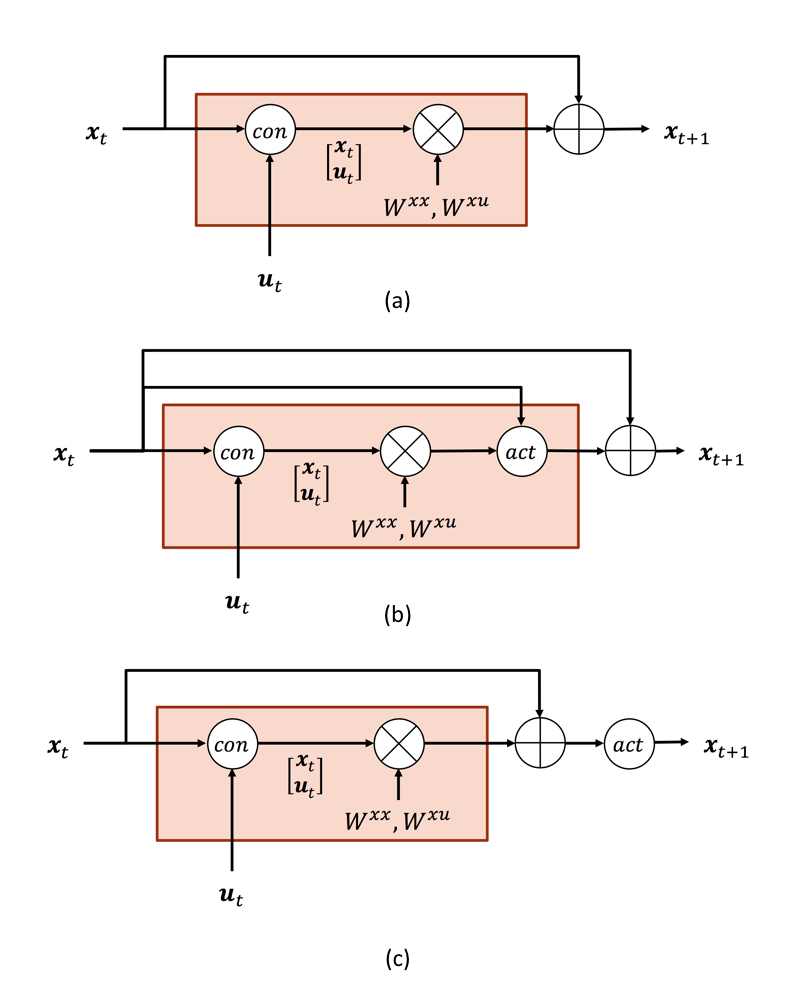
where $$$\Delta t$$$ is the time interval between adjacent time points. The neural equation can be rewritten into a piece of G-RNN and visualized as in Fig. 1 (a)
$$\begin{align}\mathbf{x}_{t+1} & \approx \Delta tA\mathbf{x}_t + \Delta tC\mathbf{u}_t + \mathbf{x}_t\ \\& =\begin{bmatrix}\Delta tA & \Delta tC\end{bmatrix}\begin{bmatrix}\mathbf{x}_t\\ \mathbf{u}_t\\\end{bmatrix} + \mathbf{x}_t\\&\equiv \begin{bmatrix}W^{x x} & W^{x u}\end{bmatrix}\begin{bmatrix}\mathbf{x}_t\\ \mathbf{u}_t\\\end{bmatrix} +\mathbf{x}_t\end{align}$$
$$$x_n,n\in \{1,2,...,N \}$$$ is a scalar abstract description of the neural activity in the n-th brain region. Its closest biophysical meaning is the average neuron firing rate of a region. No matter in the simplified Eq. (1) or the more standard bilinear form, the neural equation is largely linear. A sigmoid-shaped function is a more appealing candidate for the neuron firing model, the relationship between input stimuli and region average neuron firing rate10,11: neurons largely stay inactivated until the stimuli pass an intensity threshold and neuron firing saturates under very strong stimuli. The sigmoid-shaped neuron firing model, or even more complex ones, can be incorporated into DCM-RNN as an activation function as in Fig. 1 (b), which modifies increments of $$$x$$$. Relu12 activation provides a practical simplification of the sigmoid-shaped neuron firing model as clinical evidence shows that percentage of neurons activated as a certain time is between 1% to 4%13, far away from saturation. Relu assumes no neuron firing when the stimuli are below an intensity threshold and a linear relationship between the stimuli and neuron firing when the stimuli are above the intensity threshold. For relu activation, a simple structure as in Fig. 1 (c) can be used. As long as the activation is partial differentiable, the addition basically requires no modification to the back-propagation-based estimation in DCM-RNN.
Methods and Results
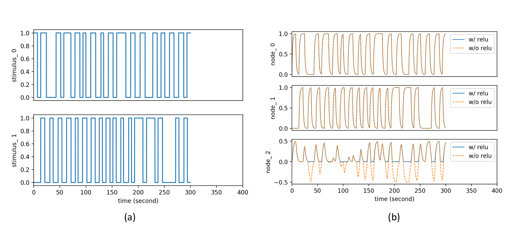
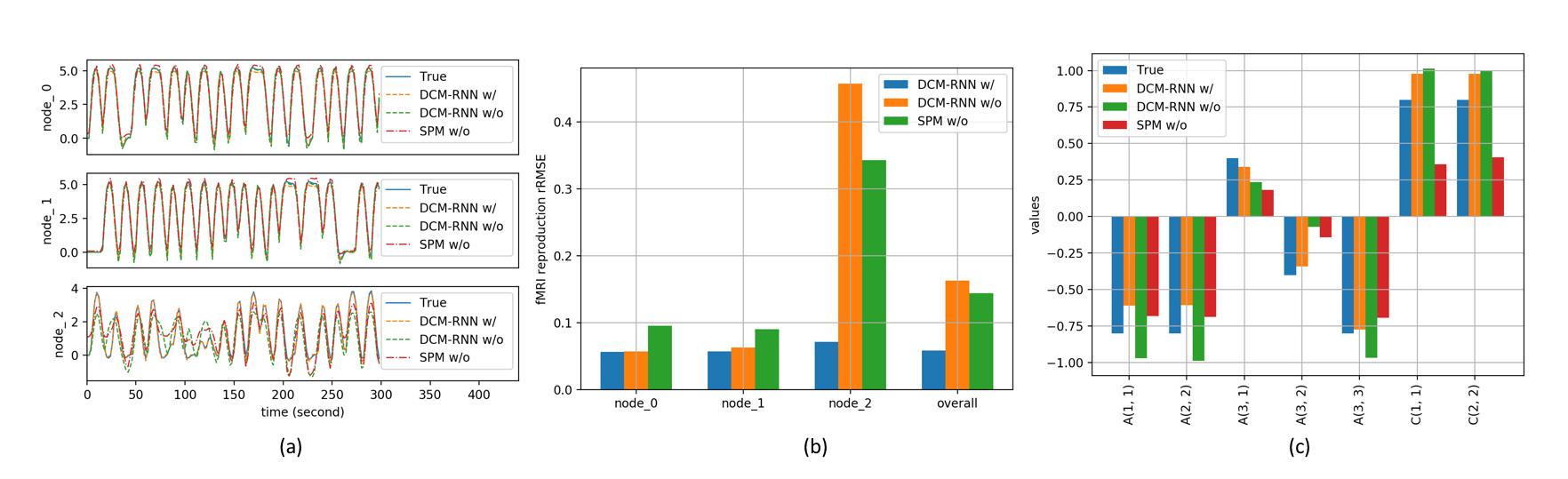
To demonstrate the importance of the added activation, we conduct an effective connectivity estimation experiment with simulated data. Data are simulated by DCM-RNN since it is more accurate than the classical DCM5. The simulation uses standard relu activation with the inflection point at 0. The effective connectivities are set as in Fig. 2 and the stimuli are randomly created. Three estimations are made and compared: DCM-RNN with relu, DCM-RNN without relu, and the classical DCM. We run Statistical Parametric Mapping (SPM) for classical DCM and no relu activation option is available. The simulated data are shown in Fig. 3 and the estimation results are shown in Fig. 4.Discussion
If the neuron firing behavior can be fairly modeled by the relu activation, ignoring it may degrade estimation significantly, as reflected by substantially increased signal reproduction error in node 3 and errors in links to node 3.Conclusion
Here we take advantage of the flexibility of DCM-RNN, easily incorporating a neuron firing model into DCM. The incorporation of neuron firing may significantly impact effective connectivity estimation.Acknowledgements
This work was supported in part by R01 NS039135-11 from the National Institute for Neurological Disorders and Stroke (NINDS) and was performed under the rubric of the Center for Advanced Imaging Innovation and Research (CAI2R, www.cai2r.net), a NIBIB Biomedical Technology Resource Center (NIH P41 EB017183).References
- Friston KJ, Harrison L, Penny W. Dynamic causal modelling. Neuroimage 2003; 19(4):1273–1302.
- Smith SM. The future of FMRI connectivity. Neuroimage 2012; 62(2):1257–1266.
- Smith SM, Vidaurre D, Beckmann CF et al. Functional connectomics from resting-state fMRI. Trends Cogn. Sci. 2013; 17(12):666–682.
- Wang Y, Wang Y, Lui YW. Generalized Recurrent Neural Network accommodating Dynamic Causal Modelling for functional MRI analysis. ISMRM, 2017.
- Wang Y, Wang Y, Lui YW. Generalized Recurrent Neural Network accommodating Dynamic Causal Modelling for functional MRI analysis. Submitted to NeuroImage .
- Friston K, Mattout J, Trujillo-Barreto N et al. Variational free energy and the Laplace approximation. Neuroimage 2007; 34(1):220–234.
- Friston KJ, Trujillo-Barreto N, Daunizeau J. DEM: A variational treatment of dynamic systems. Neuroimage 2008; 41(3):849–885.
- Friston KJ. Variational filtering. Neuroimage 2008; 41(3):747–766.
- Friston KJ. Functional and effective connectivity: a review. Brain Connect. 2011; 1(1):13–36.
- Marreiros AC, Kiebel SJ, Friston KJ. Dynamic causal modelling for fMRI: A two-state model. Neuroimage 2008; 39(1):269–278.
- Wilson HR, Cowan JD. A mathematical theory of the functional dynamics of cortical and thalamic nervous tissue. Biol. Cybern. 1973; 13(2):55–80.
- Glorot X, Bordes A, Bengio Y. Deep Sparse Rectifier Neural Networks. Aistats 2011; 15:493–497.
- Lennie P. The cost of cortical computation. Curr. Biol. 2003; 13:507–513.
Figures