0414
Deep CEST MRI – 9.4T spectral super-resolution from 3T CEST MRI data1High-Field Magnetic Resonance, Max Planck Institute for Biological Cybernetics, Tuebingen, Germany, 2X, Mountain View, CA, United States, 3Diagnostic & Interventional Neuroradiology, University Hospital Tuebingen, Tuebingen, Germany
Synopsis
CEST peaks are easy to detect at ultra-high-field strengths due to high signal and spectral separation. However, spectral coalescence and line broadening makes modeling of CEST effects at clinical field strengths (<=3T) a challenge. In this proof-of-concept study of super-resolution CEST imaging, the underlying spectral features of 3T Z-spectra were predicted using a neural network trained on 9.4T data. Applying the neural network to untrained volunteer and patient data acquired at 3T resulted in the expected contrast in healthy gray and white matter and tumor tissue in Z-spectra and APT, NOE, and MT CEST maps.
Purpose
Separating chemical exchange saturation transfer (CEST) dips in the Z-spectrum is a challenge, especially at clinical field strengths (<=3T) where amide, amine, and NOE peaks coalesce with each other or with the water peak. While Lorentzian peak separations are very successful at ultra-high fields, the broad peaks are relatively hard to isolate at 3T. The purpose of this work is to investigate if the information that is embedded in the 3T spectra can be extracted by a deep learning approach by training with 9.4T human brain target data.Methods
High-resolution Z-spectra of the same volunteer were acquired by 3D-snapshot GRE CEST MRI1 at 3T (53 offsets) and 9.4T (95 offsets). 9.4T-Z-spectra were fitted pixel-wise by a multi-Lorentzian fit2 which yields a vector of optimized multi-Lorentzian parameters, popt, containing spectral position, width and amplitude of each CEST-Lorentzian. The volume-registered 3T Z-spectra-stack was then used as an input for a 3-layer deep neural network (NN, 400 neurons total) with the volume-registered 9.4T popt-stack as target values. The 9.4T Z-spectrum is approximated from the multi-Lorentzian popt output for validation. The dataset was divided randomly into training (70%), validation (15%), and test sets (15%) to avoid overfitting. Trained with about 1000 iterations, the NN was applied to training data and to untrained from two subjects scanned at 3T.Results
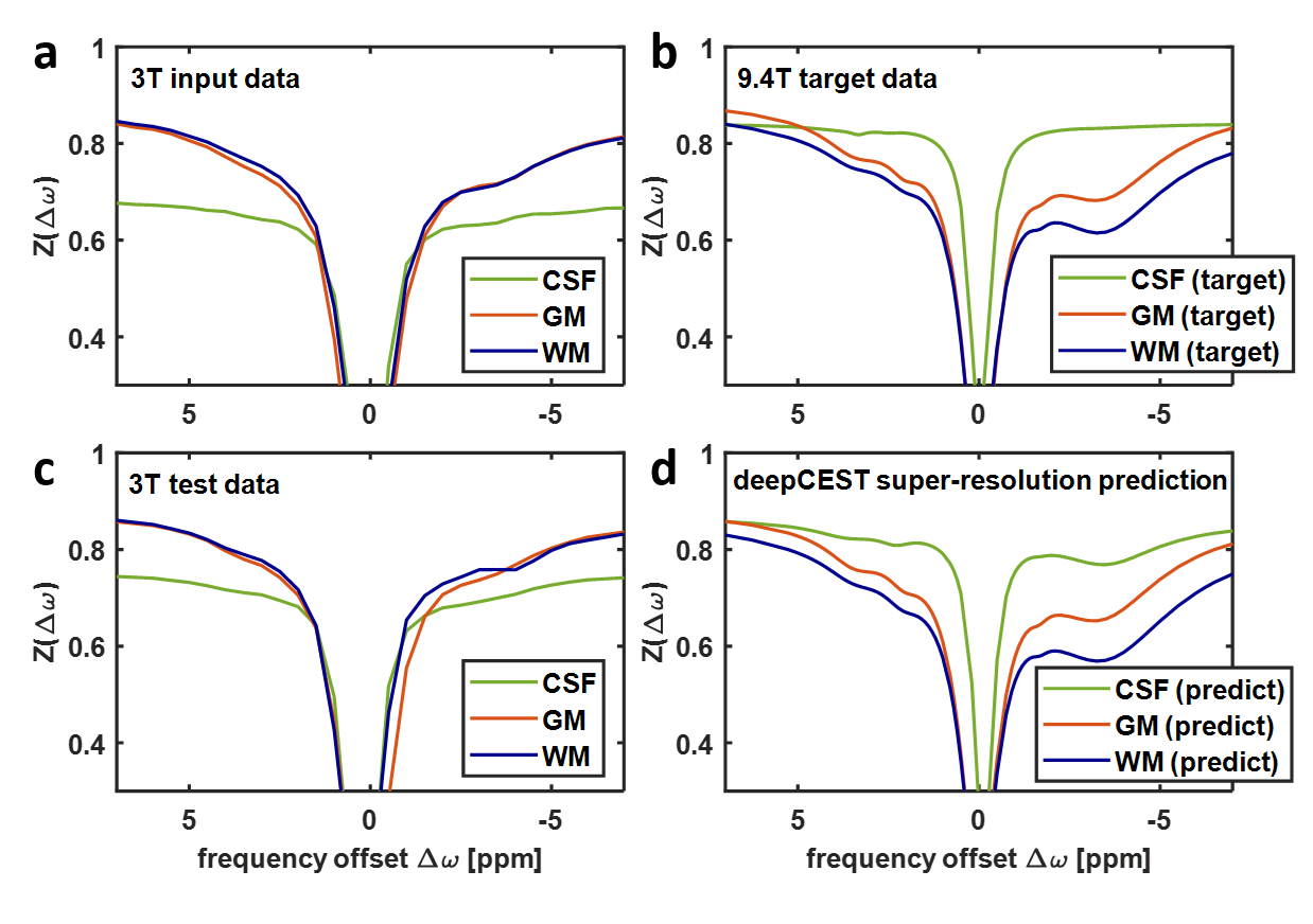
Figure 1 shows the input (a) and target (b) data of the co-registered 3T and 9.4T training datasets, the untrained data of a different volunteer (c) and the 9.4T NN prediction (d). The 3T spectral features (more pronounced NOE dip in white matter at -3.5ppm, and slightly more pronounced amide dip in gray matter at 2ppm) nicely transfer to the generated 9.4T Z-spectra. There are features at -1.7ppm and 2ppm in the deepCEST Z-spectra that are not at all visible in the original 3T data.
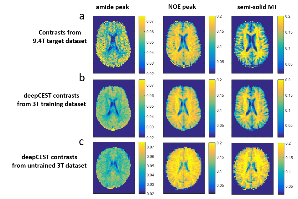
Figure 2 shows CEST maps with the target contrast from 9.4T training data (first row). Predicted maps the 3T training data (second row) show lower contrast but consistent results. Application of the trained neural network to completely new data from a different volunteer appears to generate super-resolved contrasts with the same GM/WM features for the individual resonances.
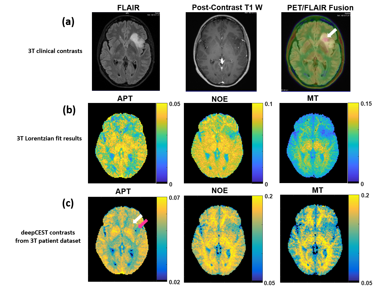
Applying the NN to 3T data from a brain tumor patient (Figure 3) showed that the 9.4T-contrast prediction also revealed similar decreases of NOE, APT, and MT effects in the tumor as observed by direct evaluation of 3T Z-spectra. Predicted elevated APT signals also match the FET-PET hyperintesity (white arrow).
Discussion
We were surprised by the astounding results of just a single volunteer data set. Stable neural network training requires a large amount of data. With the high spectral-spatial resolution and 3D volume coverage of snapshot-CEST, 209000 Z-spectra from the healthy human brain were available for training.
This is to our knowledge the first application of machine learning to CEST data. Thus more questions than answers arise right now. The answers first:
- The principle GM/WM/CSF contrast of predicted NOE/APT/MT could be shown, thus the approach is feasible and does not produce random predictions.
- The predicted
data looks smooth, indicating that the neural network might also be a smart de-noising
algorithm for CEST data. Note that no spatial information was
used for the training of the neural network. The spatially smooth prediction is a
surprising result.
- Without training on pathology, the deepCEST approach was able to predict CEST contrasts in tumor tissue with similar correlations compared to the directly evaluated data and the tumor could be outlined.
The open questions are numerous. To just name a few:
- Does the smoothness of the predicted data also hint that some features might be lost?
- Which information did the neural network actually use? Is it only some kind of segmentation, an average Z-spectrum value, or really the meaningful CEST offsets?
- Will this translate to completely untrained data, e.g. tumors or other pathological tissue with Z-spectra of completely different shape?
- Is the prediction of peaks that are clearly visible at 9.4T but almost invisible at 3T (e.g. 2 ppm or -1.7 ppm) random or a good estimation?
While some of these questions can be answered by investigating the trained net in detail, others must be validated in larges studies. Increasing the training, validation, and test datasets for healthy volunteers and pathologies is a necessary next step. This study is ongoing, with scanning of patients at both field strengths.
Conclusion
Machine learning might be a powerful tool for CEST data processing and could bring the benefits and insights of the few ultra-high field sites to a broad clinical use. Such approaches must be handled with care if pathologies are evaluated.Acknowledgements
The financial support of the Max Planck Society, German Research Foundation (DFG, grant ZA 814/2-1, support to M.Z.), and European Union’s Horizon 2020 research and innovation programme (Grant Agreement No. 667510, support to M.Z.) is gratefully acknowledged.References
- Zaiss et al. “snapCEST – A single-shot 3D CEST sequence for motion corrected CEST MRI.” Proc. ISMRM 2017, p. 3768.
- Windschuh et al. “Correction of B1-inhomogeneities for relaxation-compensated CEST imaging at 7T.” NMR in Biomed 2015; 28:529-537.
Figures