Motivation and Clinical relevance:

The availability of homogeneous magnetic field (<5ppm) is a critical component in modern day MR scanners to achieve clinically acceptable images. This stringent requirement escalates the expense of the superconducting magnet and hence the price of the MR machine. Reduction and/or relaxation of this constraint would have a significant impact on cost and access, resulting in increased MR value. The REMODEL method allows for reconstruction of MR images with comparable image quality to Ground Truth (GT), in the presence of high off resonance artifacts ranging up to ±50kHz.

Impact:

The cost of the MR machine can be reduced by utilizing REMODEL for reconstruction of images resulting from a magnet designed with lower homogeneity constraints. REMODEL can address off resonance artifacts at varying field strengths¹ of 1.5T and Ultra High Fields (UHF) MRI. The usage of only matrix multiplications for reconstructing test data in REMODEL is expected to result in accelerated computational time.

Approach:

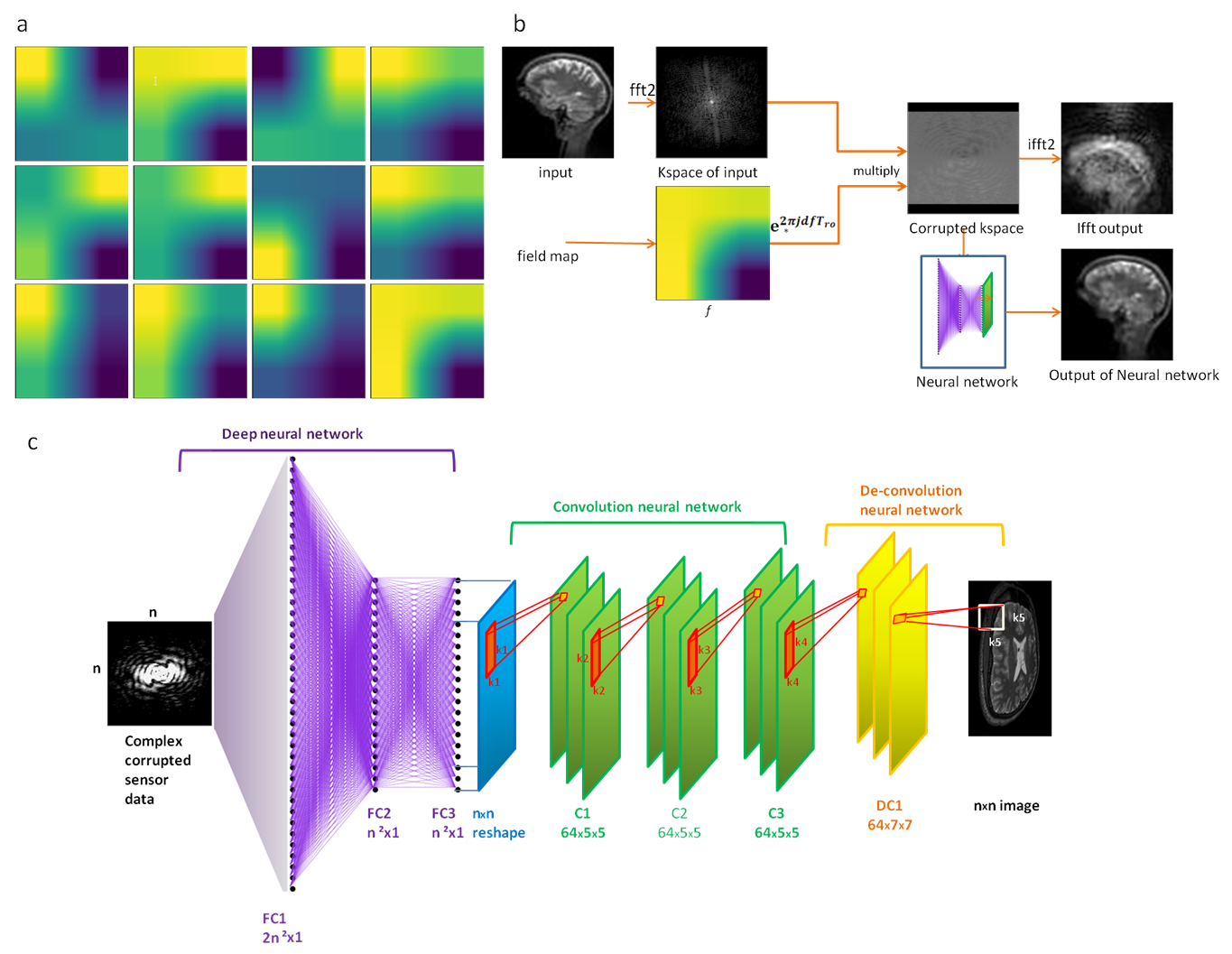
Data collection and pre-processing for retrospective inhomogeneous field reconstruction: Sagittal T1 weighted and MPRAGE images from 70 subjects were collected from the Human Connectome Project (HCP)² for training the neural network. These were then converted to axial and coronal images using MeVis Lab (Fraunhofer MeVis, Germany) to train for different orientations. All these images were rotated in 90o increments to augment the data set to generate 32000 images. Off resonance artifacts were introduced by generating 12 random field maps by creating a random 2x2 matrix which was then extrapolated to cover the complete image area creating a smooth sinusoids³ as shown in figure 1a. These field maps were normalized between -1 to 1 and then multiplied by different off-resonance ranges. Here, we assumed a read out time of 4.96ms. The training data was prepared by multiplying the kspace of the image with one of twelve randomly selected off resonance phase maps (figure 1b).
Model architecture: The neural network used for training has 3 fully connected layers, 3 convolution layers followed by one deconvolution layer, similar to the network in ref 4. Tensorflow (Google Inc, USA) was the computational frame work employed to train this neural network. The kspace (nxn complex) was then reshaped to 2n²x1 real valued vector and given as input to first fully connected layer (FC1). The architecture is detailed in figure 1c. All layers were activated by Relu activation function.
Training details: We trained the network using images of size 32x32 and 64x64 with an off-resonance frequency range of ±10kHz, and ±30k and ±50kHz respectively. Adam optimizer was used with mini batches of size 128, learning rate 10^-4. We used Xavier initialization for weights and applied mini batch normalization across layers. The loss function used for training was mean squared loss between the network output and target image intensity values with an additional L₂ norm and regularization value of λ=10^-3. Each network was trained for 600 epochs using 2 GetForce GTX 1080 Ti GPUs with 11GB memory capacity each. The performance of the resulting network was tested using the images downloaded from HCP that were not included for training, corrupted with random field maps.

Preliminary Data:

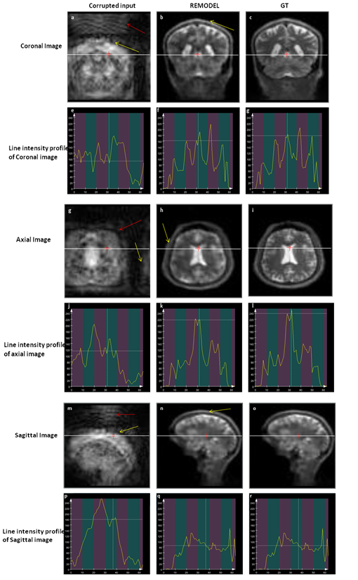
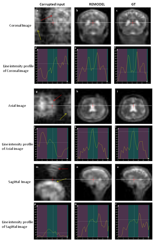
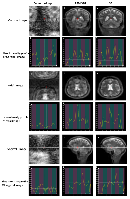
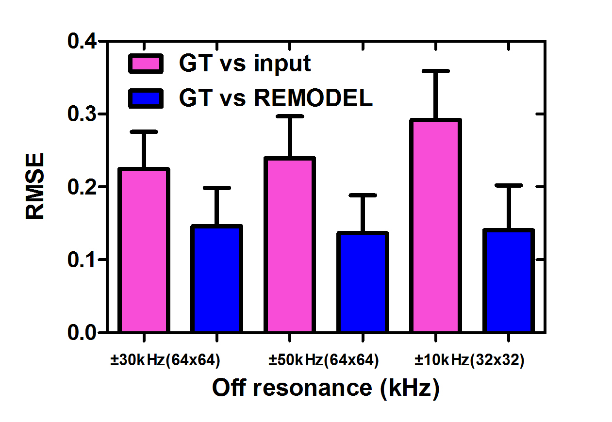
Figure 2a shows the 64x64 coronal image corrupted by ±30kHz off-resonance. The figure shows the blurring (red arrow) and pixel shifting (yellow) due to inhomogeneity. It can be observed in figure 2b that these artifacts are significantly removed by REMODEL. The line intensity profiles in figure 2d are similar to those shown for GT. Analogous results can be seen in axial and sagittal orientations in figure 2. Figures 3 and 4 show the results of REMODEL reconstructions for dimensions of 32x32 and 64x64 images corrupted by ±10kHz and ±50kHz respectively. The average and standard deviation of the Root Mean Square Error plot of over 190 examples in figure 5 quantitates the reduction of artifacts by REMODEL reconstruction with reference to the GT, as compared to the corrupted images.

Gains and Losses:

REMODEL has been demonstrated on synthetically corrupted data from a publicly available database. It is able to faithfully reconstruct the images simulated in inhomogeneous fields up to ±50kHz, which can be extended to higher off-resonance ranges without any change in implementation details. Implementation details along with source code can be found online5. The model has been trained for brain MRI datasets and for a fixed readout time. However, this can be easily extended to other body regions and for multiple readout times. The results have been demonstrated on smaller dimensions due to available computation facilities. This could be overcome with higher compute power.

Acknowledgements

This work was supported by grant funding from DST/VGST/KFIST/LII/GRD333.