0295
Workflow proposal for defining SAR safety margins in parallel transmission1NeuroSpin, CEA, Saclay, France, 2Irfu, CEA, Saclay, France
Synopsis
SAR calculations in parallel transmission (pTx) typically rely on electromagnetic simulations performed on generic models. Uncertainties however often exist due to tolerances in the lumped element values, cable losses, phase offsets and different coupling between transmit elements. Additional uncertainties in SAR evaluation include intersubject variability and exam supervision. In this work, we review a workflow that has been implemented in our laboratory with home-made and commercial pTx coils at 7T. Based on this strategy, nearly 100 healthy volunteers have been scanned with no reported incidents, while still allowing to exploit pTx to mitigate efficiently the RF inhomogeneity problem.
Purpose
SAR calculations in parallel transmission typically rely on numerical simulations performed on generic models. To enable accurate and safe local SAR supervision, model imperfections inherent to this approach need to be identified and quantified. In this work, we propose a workflow to accomplish this task.Methods
The strategy consists of analyzing three fundamental uncertainties leading to three (concatenated) individual safety factors applied to the SAR prediction and incorporated into Virtual Observation Points (VOP)1 matrices provided to the scanner for real-time supervision.
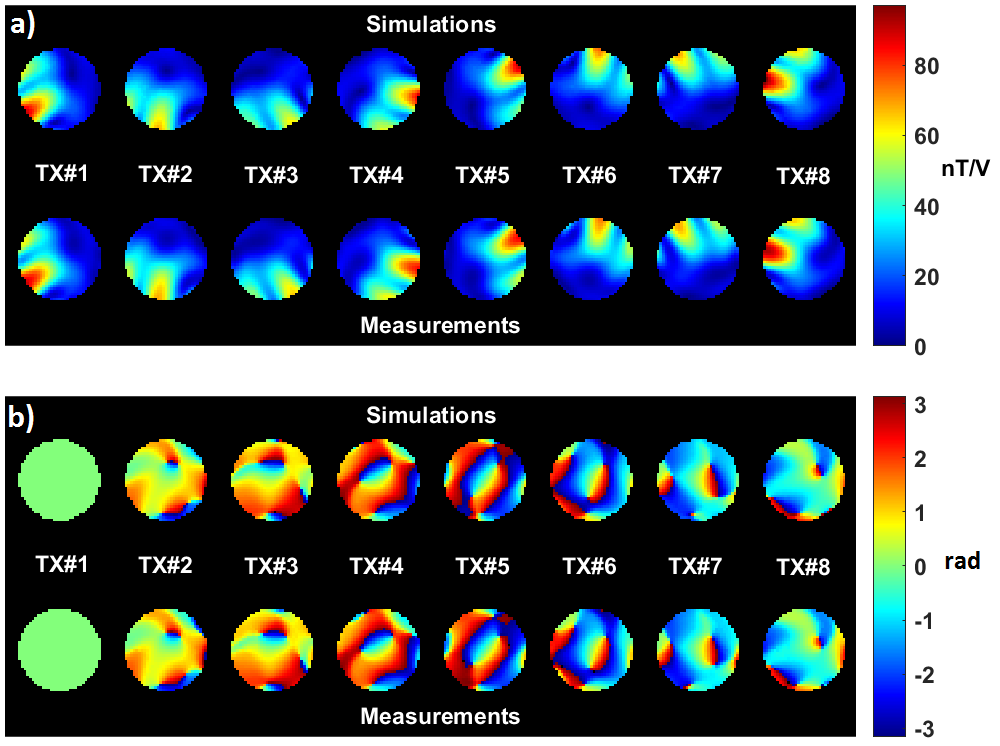
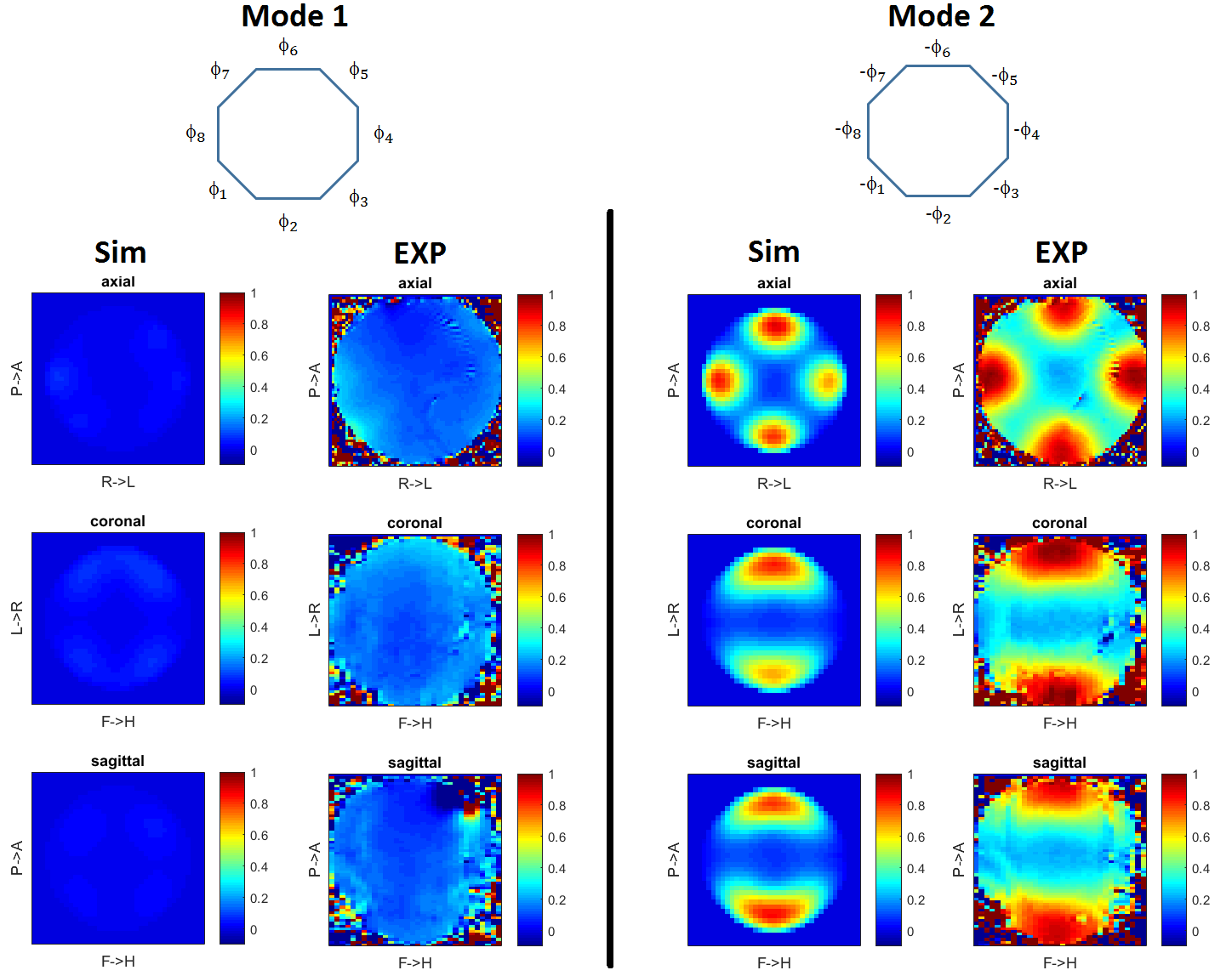
Coil modelling: SAR margins related to imperfect coil modelling are computed for a phantom of known geometry, electric properties and position. Our reference phantom is a 16 cm diameter spherical agar-gel phantom with 4 g/l NaCl (σ=0.78 S/m and εr=72 at 298 MHz). Electromagnetic simulations are performed with appropriate software after tuning/matching the array in the numerical domain2. Transmit B1 maps are measured and compared to the simulated ones. For unaccounted cable losses, phase offsets and different coupling, as demonstrated elsewhere3,4 simulated electromagnetic fields can be tuned by appropriate linear combinations. Thus we calibrate our B1 simulations by fitting each measured complex B1 map as a linear combination of the simulated ones. For the kth transmit channel, one obtains $$$B_{1,k}^{measured}\approx B_{1,k}^{cal}=\sum_{n=1}^N \alpha_{k,n} B_{1,n}^{sim}$$$, where N is the number of channels and [αij] is the so-called calibration matrix, which likewise returns calibrated electric fields. The remaining discrepancy between the measured and simulated B1 maps is quantified and propagated into a SAR amplification factor5. MR thermometry is performed on the phantom for two modes of excitation to control that the peak measured temperature rise is within the computed margin and that the heating patterns match. The calibration matrix, determined with phantom data, is then applied to the generic head model E-field simulations. This extrapolation is rigorous when involving cable-related phase offsets and losses, while uncertainties in the tuning/matching variations of the transmit coil are taken into account in the intersubject variability factor. The calibration matrix with the reference phantom is controlled each day in-vivo experiments are scheduled to control any possible fault that could impact the SAR calculations6.
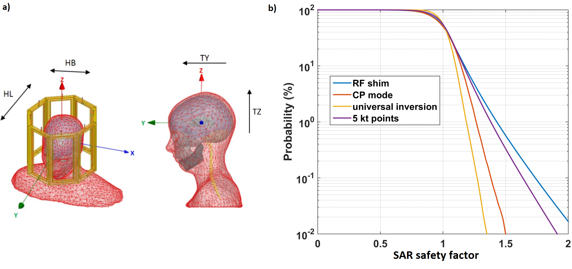
Intersubject variability: EM simulations are generally performed on generic models. As a result, we have proposed a statistical analysis to assess the sensitivity of the SAR with respect to different parameters such as head length, head width and position7. If the SAR behavior is smooth enough for small variations, knowing the statistics8 of the different parameters allows calculating the output SAR statistics7, the latter being pulse-dependent. Safety factors can then be determined based on risk analysis.
Exam supervision: Real-time supervision based on directional couplers (Dico) incorporates uncertainties in the amplitude and phase of the transmit RF voltage (in our case 10 % and 5°). To address this, we maximize the SAR for many random RF pulses based on this uncertainty, to return a last SAR amplification factor.
Results
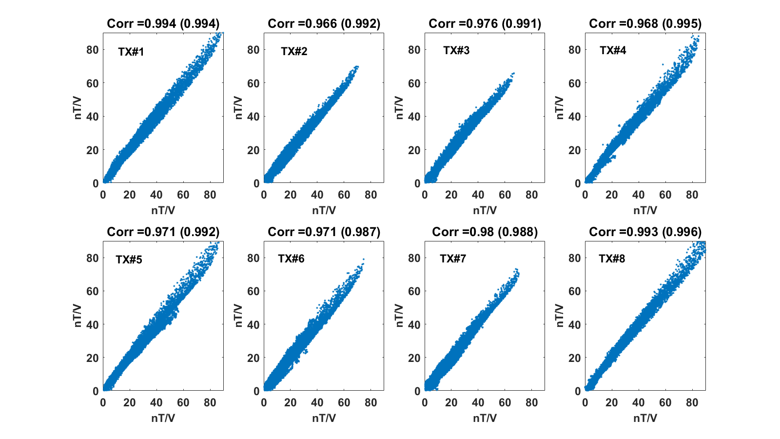
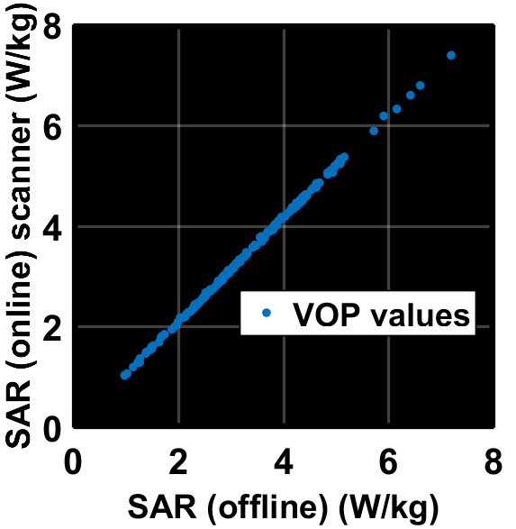
Illustrations are provided for the 8Tx-8Rx Rapid-Biomed head coil (Rapid-Biomedical, Rimpar, Germany) at 7T. Figure 1 shows the resulting calibrated B1 simulations versus the measured ones, while Figure 2 reports the correlations and corresponding scattered plots. Root mean square error between the two is ~2.1 nT/V and results into a ~1.25 SAR amplification (safety factor) of the peak 10g SAR5, consistently with the MR thermometry measurements (Fig. 3). For intersubject variability, a safety margin of 1.5 was determined to have less than 1% probability for the true SAR to exceed the raised value for a random subject (Fig. 4). But due to the extra care cautioned by the IEC9, an additional safety factor of 2 is taken for the eye voxels only. Finally, the maximization of the SAR based on Dico uncertainties yielded a factor of 1.25, hence yielding an overall safety factor of 1.25×1.5×1.25 ≈ 2.3. Comparisons of SAR predictions versus online SAR values are presented in Fig. 5.Discussion and conclusion
This work summarizes the workflow used so far in our laboratory for pTx SAR evaluations in vivo. Based on this strategy, we have scanned nearly 100 adult volunteers over the last 2 years without any reported incident, yet in the IEC normal mode of operation. Multiplying the different safety factors can be argued to be conservative as the probability of each separate worst-case event is small. For further performance, one of the factors above could be lowered with e.g. better simulations, less Dico-uncertainties, subject-based SAR models or temperature considerations10. Another option would be to use the first level controlled mode of the IEC with twice as much 10g SAR limits.Acknowledgements
ERC EXPAT (grant number 309674).References
[1] G. Eichfelder and M. Gebhardt. Local specific absorption rate control for parallel transmission by virtual observation points. Magn Reson in Med 66:1468-1476 (2011).
[2] M. Kozlov and R. Turner. Fast MRI coil analysis based on 3-D electromagnetic and RF circuit co-simulation. J of Magn Reson 200:147-152 (2009).
[3] A. Beqiri, J. W. Hand, J. V. Hajnal and S. J. Malik. Comparison between simulated decoupling regimes for SAR prediction in parallel transmit MRI. Magn Reson in Med 74:1423-1434 (2015).
[4] P. Vernickel, C. Findeklee, J. Eichmann and I. Graesslin. Active digital decoupling for multi-channel transmit MRI systems. Proc of the 15th ISMRM meeting, p 170 (2007).
[5] G. Ferrand, M. Luong, A. Amadon and N. Boulant. Mathematical tools to define SAR margins for phased array coil in-vivo applications given E-field uncertainties. Proc of the 23rd ISMRM meeting, p 3763 (2015).
[6] J. Hoffmann, A. Henning, I. A. Giapitzakis, K. Scheffler, G. Shajan, R. Pohmann and N. Avdievich. Safety testing and operational procedures for self-developed radiofrequency coils. NMR in Biomed 29:1131-1144 (2016).
[7] M. Le Garrec, V. Gras, M-F Hang, G. Ferrand, M. Luong and N. Boulant. Probabilistic analysis of the specific absorption rate intersubject variability safety factor in parallel transmission MRI. Magn Reson in Med 78:1217-1223 (2017).
[8] R. Ball, C. Shu, P. Xi, M. Rioux, Y. Luximon, J. Molenbroek. A comparison between chinese and caucasian head shapes. Applied Ergonomics 41:832-839 (2010).
[9] International Electrotechnical Commission. Medical equipment part 2-33: particular requirements for the basic safety and essential performance of magnetic resonance equipment for medical diagnosis. 3rd ed. Geneva: International Electrotechnical Commission 2011;601:2-33.
[10] N. Boulant, X. Wu, G. Adriany, S. Schmitter, K. Uğurbil and P-F Van de Moortele. Direct control of the temperature rise in parallel transmission by means of temperature virtual observation points: Simulations at 10.5 tesla. Magn Reson in Med 75:249-256 (2016).
Figures