0254
Effect of combining linear with spherical tensor encoding on estimating brain microstructural parameters1Radiology, New York University School of Medicine, New York, NY, United States, 2Clinical Sciences, Lund University, Lund, Sweden, 3Random Walk Imaging AB, Lund, Sweden
Synopsis
The diffusion MRI signal, as measured with conventional linear tensor encoding (LTE), has been shown to have not enough features to fully model the white matter microstructure. Here we investigate whether adding spherical encoding (STE) to LTE makes microstructural parameter estimation more robust. On signal simulations and in in vivo MRI data, we demonstrate that the intra-axonal diffusivity and axonal water fraction are estimated with higher precision, thereby enabling a 20 minute whole brain protocol to extract brain microstructural parameters without imposing constraints or priors.
INTRODUCTION
Diffusion MRI (dMRI) is the method of choice to probe cellular architecture at a level far below the millimeter MRI resolution, yet biophysical modeling is warranted to extract specific microstructural features. In brain, the biophysical Standard Model1 consists of impermeable sticks (representing axons, possibly glial cells) embedded in the extra-axonal compartment. Unfortunately, the dMRI signal, as commonly obtained by applying diffusion gradients along single directions2, also known as linear tensor encoding (LTE), does not contain enough features to extract the standard model parameters robustly.3,4 Here, we combine the conventional LTE with isotropic or spherical tensor encoding (STE)5, and investigate how the Standard Model parameter estimation benefits from the complementarity of both schemes.METHODS
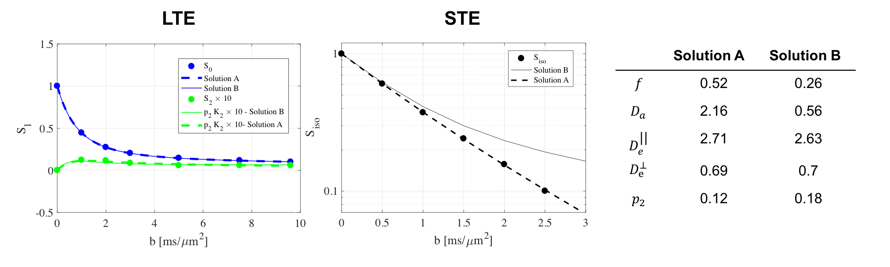
Theory The Standard Model for the diffusion signal $$S_{{\bf\,g}}(b)=\int_{|\mathbf{n}|=1}\!\!d\mathbf{n}\,\mathcal{P}(\mathbf{n})\,\mathcal{K}(b,{\bf\,g}\cdot\mathbf{n})\,\quad\quad(1)$$ is a convolution on a unit-sphere $$$|\mathbf{n}|=1$$$ between the fiber orientation distribution function (ODF) $$$\mathcal{P}(\mathbf{n})$$$ and the 2-compartment elementary-fiber kernel $$\mathcal{K}(b,\xi)=S_0\left[f\,e^{-bD_a\xi^2}+(1-f)\,e^{-bD_e^\perp-b(D_e^\parallel-D_e^\perp)\xi^{2}}\right]\,,\quad\quad(2)$$ parameterized by proton density $$$S_0$$$, intra-axonal-axial $$$D_a$$$, extra-axonal-axial $$$D_e^\parallel$$$ and extra-axonal-radial $$$D_e^\perp$$$ diffusivities, and axonal water fraction $$$f$$$. Convolution (2) factorizes4,6-10 in the spherical-harmonic basis, $$S_{lm}(b)=p_{lm}\,K_l(b)\,.\quad\quad(3)$$ We employ the rotational-invariant (RotInv) formalism4,6 to factor out the ODF, by introducing basis-independent rotational-invariants of the signal and ODF $$$S_l\equiv\sqrt{\sum_{m=-l}^l\,S_{lm}^2}/\mathcal{N}_l$$$, $$$p_l\equiv\sqrt{\sum_{m=-l}^l\,p_{lm}^2}/\mathcal{N}_l$$$, $$$\mathcal{N}_l=\sqrt{4\pi(2l+1)}$$$. In this way, we solve the system $$S_l(b,x)=p_l\,K_l(b,x)\,,\quad\,l=0,2\,,\quad\,p_0\equiv1\quad\quad(4)$$ for 6 unknowns: fiber-compartment-parameters $$$x=\{S_0,f,D_a,D_e^\parallel,D_e^\perp\}$$$ and ODF-anisotropy-invariant $$$p_2$$$. Nonlinear fitting (4) is generally unstable3,4,6, characterized by multiple solutions and shallow "trenches" near the fit minima. Here we evaluate the advantages of additionally employing isotropic encoding $$S_{\mathrm{iso}}(b)=S_0\left[f\,e^{-bD_a}+(1-f)\,e^{-b(D_e^\parallel+2D_e^\perp)}\right]\quad\quad(5)$$ that automatically factors-out the ODF, and senses the parameters $$$x$$$ in a different combination, as an "orthogonal" measurement to improve precision of the fit (4) for anisotropic compartments.
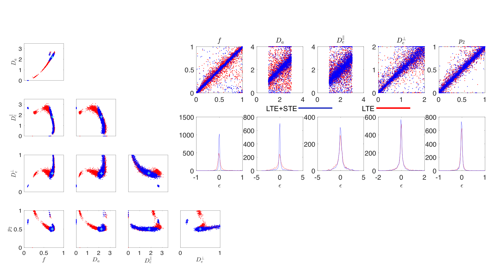
Noise Propagation analysis was performed to investigate the accuracy and precision of the joint RotInv fit (4)-(5), referred to as LTE+STE, versus the RotInv fit (4), referred to as LTE. For the acquisition protocol described below, 2500 noise realizations with SNR=100 at $$$b=0$$$, were simulated for one parameter vector (Fig 1a) as well as for a range of biologically plausible parameter vectors (Fig1b). Each fit was initiated using one random starting point sampled from: $$$0≤f≤1$$$, $$$0\leq\,p_2\leq,1$$$, $$$0\leq\,D\leq\,4\mu$$$m2/ms for all diffusivities.
Imaging Seven healthy volunteers (3 males, age range 26-35) were scanned on a 3T Siemens Prisma scanner with a 32-channel head coil. A repeated scan within 30 days was performed on 2 volunteers to evaluate scan-rescan precision. The LTE protocol (10:53 min) used the product diffusion sequence and included 165 images acquired using monopolar gradients along 30 directions for b=1000, 2000, 3000, and along 64 directions for b=5000 s/mm2, in addition to 11 b=0-images. The STE protocol (9:52min) included 70 images acquired using a prototype spin-echo sequence that enables variable shapes of the b-tensor by numerically optimized waveforms11, for b-values ranging from b = 0 up to b = 3000 in steps of 500s/mm2. Other parameters were: acquisition matrix = 70 x 70, image resolution = 3x3x3 mm2, TE=102ms, TR=3800ms, grappa 2, multiband-2 (LTE), 38 oblique axial slices. Data was denoised12 and gibbs13, eddy-current14, Rician-bias15, and B1-bias16 corrected prior to model fitting, similar as described above.
RESULTS AND DISCUSSION
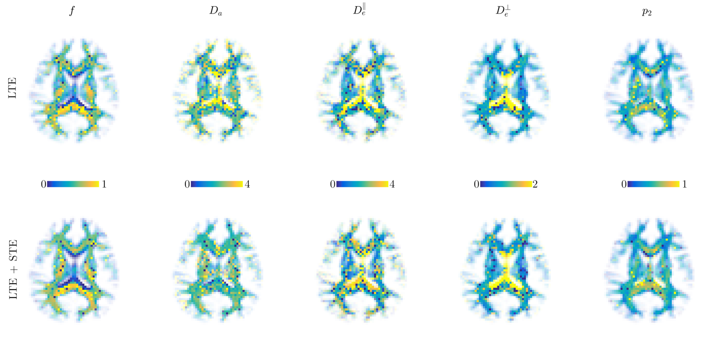
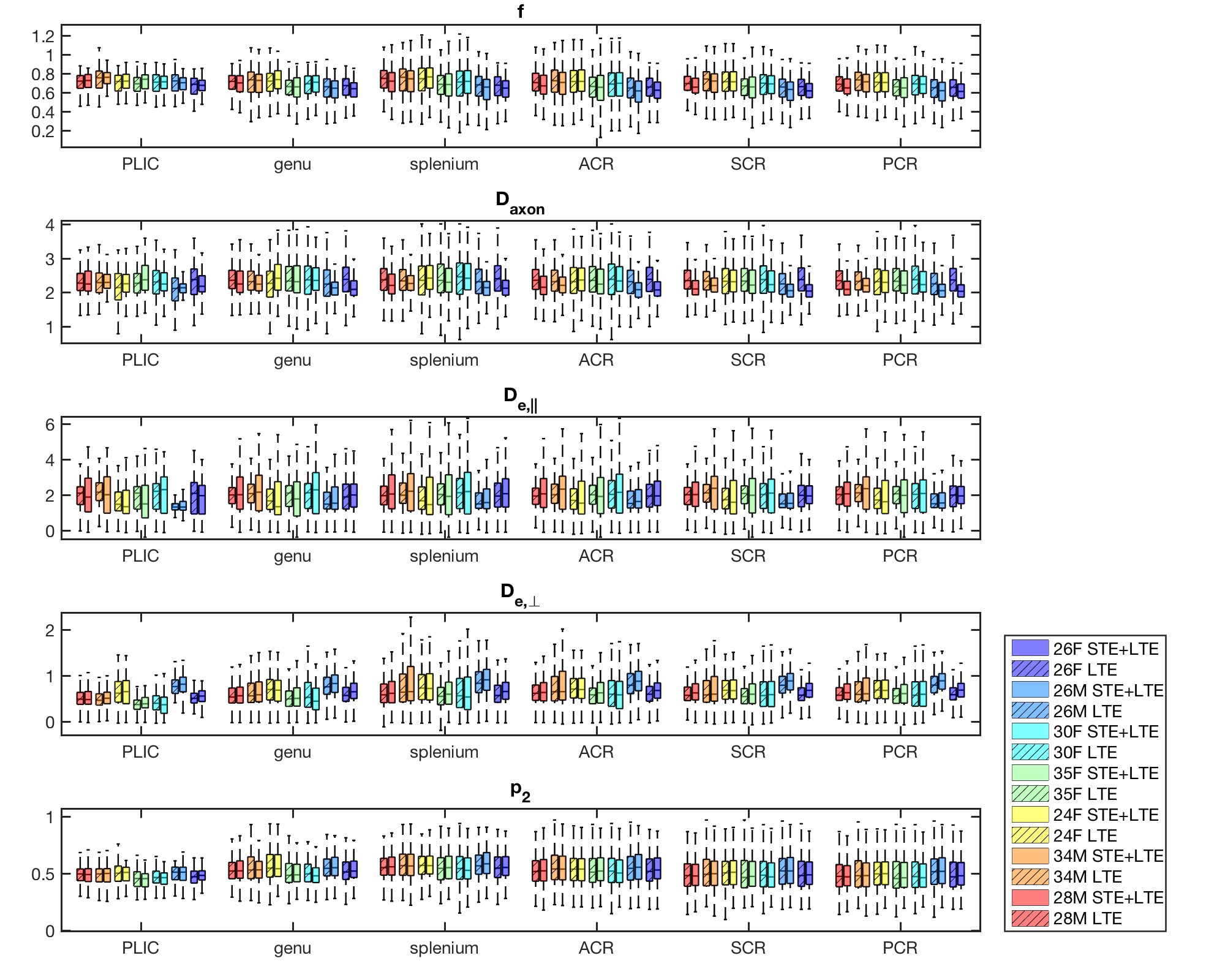
Both simulations (Fig.1) and in vivo results (Fig 2-5) corroborate the finding of increase in precision of $$$D_a$$$ , and to a lesser extent $$$f$$$, when including STE in addition to LTE in the nonlinear model fitting (4)-(5), yet the precision of the extra-axonal diffusivity decreased in the in vivo data. While multiple solutions are still present (Fig.1,4), they are better identifiable as outliers compared using LTE only, which would imply re-doing the fit with different starting point to retrieve the other solution (not included here to provide fair presentation of the pitfalls of fitting).
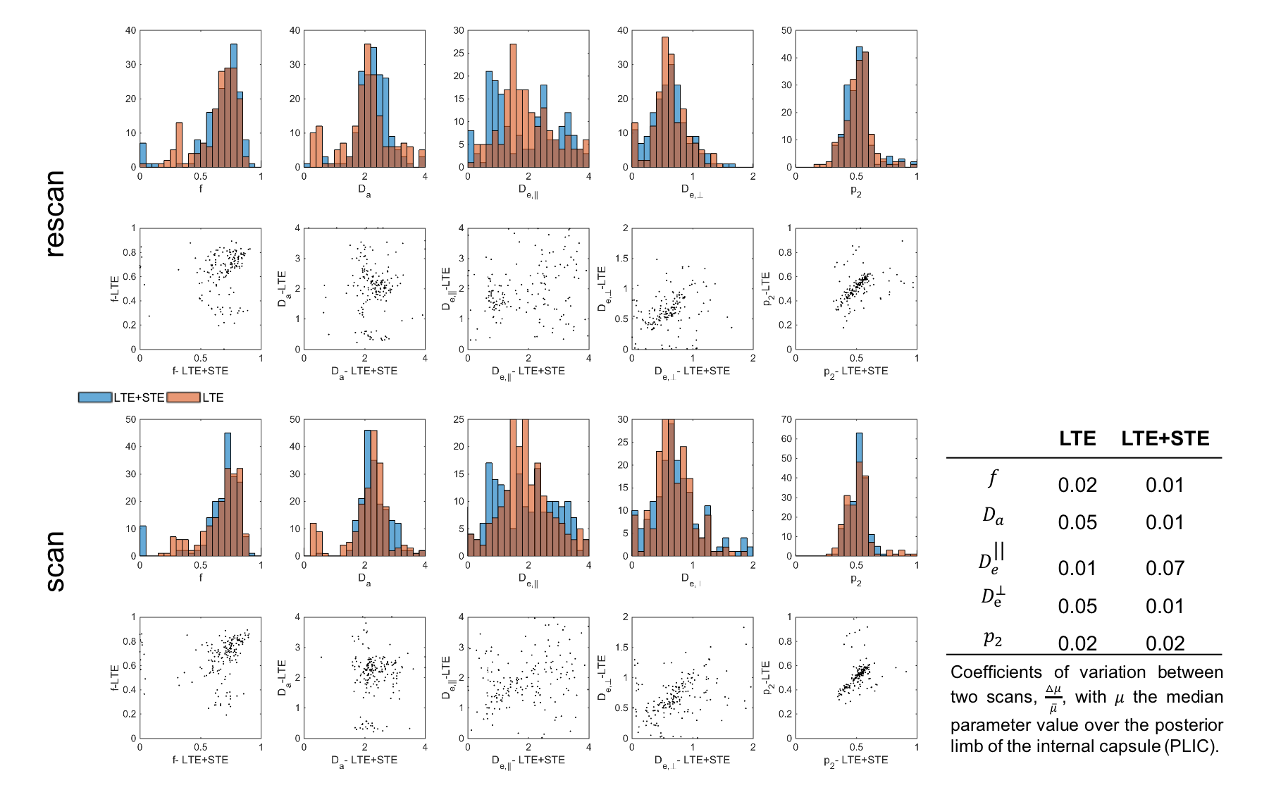
The obtained values over all WM regions of all subjects for $$$D_a=2.2\pm0.66$$$ (LTE+STE), and $$$2.17\pm0.67$$$ (LTE), are both in good agreement with reported values using other orthogonal diffusion methods.17,18 Along with increased precision of $$$D_a$$$, the scan-rescan improved, as illustrated in Fig.4 for the PLIC. While the simulations kept the total number of measurements the same, the LTE+STE data had 70 additional weightings, which can explain some of the overall improvement. Future work will focus on incorporating a free water compartment (which may affect our corpus callosum results) and extending to other “orthogonal” acquisition methods by varying, e.g., the echo17 or diffusion time.
CONCLUSIONS
Combining linear with spherical tensor encoding provides an “orthogonal” measurement dimension that enables more precise and robust estimation of the intra-axonal diffusivity and axonal water fraction. Our proposed method allows estimating all Standard Model parameters in vivo, in the whole brain, using ~20min acquisition and about 5-10min nonlinear fitting, without imposing priors or constraints.Acknowledgements
Research was supported by the National Institue of Neurological Disorders and Stroke of the National Institutes of Health under award number R01NS088040.References
1. Novikov, D. S., Jespersen, S. N., Kiselev, V. G. & Fieremans, E. Quantifying brain microstructure with diffusion MRI: Theory and parameter estimation. arXiv preprint arXiv:1612.02059 (2016).
2. Stejskal, E. O. & Tanner, J. E. Spin Diffusion Measurements: Spin Echoes in the Presence of a Time‐Dependent Field Gradient. The Journal of Chemical Physics 42, 288-292, (1965).
3. Jelescu, I. O., Veraart, J., Fieremans, E. & Novikov, D. S. Degeneracy in model parameter estimation for multi-compartmental diffusion in neuronal tissue. NMR Biomed. 29, 33-47, (2016).
4. Novikov, D. S., Veraart, J., Jelescu, I. O. & Fieremans, E. Mapping orientational and microstructural metrics of neuronal integrity with in vivo diffusion MRI. arXiv preprint arXiv:1609.09144 (2016).
5. Mitra, P. P. Multiple wave-vector extensions of the NMR pulsed-field-gradient spin-echo diffusion measurement. Physical Review B 51, 15074-15078 (1995).
6. Reisert, M., Kellner, E., Dhital, B., Hennig, J. & Kiselev, V. G. Disentangling micro from mesostructure by diffusion MRI: A Bayesian approach. NeuroImage 147, 964-975, (2017).
7. Tournier, J., Calamante, F., Gadian, D. & Connelly, A. Direct estimation of the fiber orientation density function from diffusion-weighted MRI data using spherical deconvolution. Neuroimage 23, 1176-1185,(2004).
8. Anderson, A. W. Measurement of fiber orientation distributions using high angular resolution diffusion imaging. Magn. Reson. Med. 54, 1194-1206, (2005).
9. Jespersen, S. N., Kroenke, C. D., Østergaard, L., Ackerman, J. J. H. & Yablonskiy, D. A. Modeling dendrite density from magnetic resonance diffusion measurements. Neuroimage 34, 1473-1486, (2007).
10. Dell'Acqua, F. et al. A Model-Based Deconvolution Approach to Solve Fiber Crossing in Diffusion-Weighted MR Imaging. IEEE Transactions on Biomedical Engineering 54, 462-472, (2007).
11. Sjölund, J. et al. Constrained optimization of gradient waveforms for generalized diffusion encoding. J. Magn. Reson. 261, 157-168, (2015).
12. Veraart, J. et al. Denoising of diffusion MRI using random matrix theory. Neuroimage, doi:http://dx.doi.org/10.1016/j.neuroimage.2016.08.016.
13. Kellner, E., Dhital, B., Kiselev, V. G. & Reisert, M. Gibbs-ringing artifact removal based on local subvoxel-shifts. Magn. Reson. Med. 76, 1574-1581 (2016).
14. Andersson, J., Jenkinson, M. & Smith, S. in FMRIB Technial Report TR07JA2 (FMRIB, Oxford, 2007).
15. Koay, C. G. & Basser, P. J. Analytically exact correction scheme for signal extraction from noisy magnitude MR signals. J. Magn. Reson. 179, 317-322, (2006).
16. Zhang, Y., Brady, M. & Smith, S. Segmentation of brain MR images through a hidden Markov random field model and the expectation-maximization algorithm. IEEE Trans. Med. Imaging 20, 45-57, (2001).
17. Veraart, J., Novikov, D. S. & Fieremans, E. TE dependent Diffusion Imaging (TEdDI) distinguishes between compartmental T2 relaxation times. Neuroimage, (2017).
18. Veraart, J., Fieremans, E. & Novikov, D. S. Universal power-law scaling of water diffusion in human brain defines what we see with MRI. arXiv preprint arXiv:1609.09145 (2016).
Figures