Synopsis

Quantitative T1ρ imaging usually requires multiple spin-lock times to obtain T1ρ maps, which makes the acquisition time demanding especially for biexponential models. Compressed Sensing has demonstrated significant acquisition time reduction in MRI. Similar improvements are expected for T1ρ relaxation mapping, given the extensive correlations in the series of images. However, it is not clear which combination of sparsifying transform and regularization function performs best for biexponential T1ρ mapping. Here, we compare five CS approaches: l1-norm of principal component analysis, spatio-temporal finite differences, exponential dictionaries, low rank, and low rank plus sparse. Our preliminary results, with three datasets, suggest that L+S is the most suitable method with least T1ρ estimation error.

Introduction:

Methods:

The CS problem is:

$$x=\arg\min_x ||m-SFCx||_2^2+λR(x).$$

Where $$$x$$$ represents the series of images (different TSLs), $$$C$$$ is the coil sensitivities, estimated using³, $$$F$$$ represents the spatial FFT, $$$S$$$ is the sampling pattern⁴ and $$$λ$$$ is the regularization parameter, adjusted for best reconstruction similarity with the reference method (SENSE coil combination⁵ using fully sampled data).

For sparsity in the principal component analysis (PCA) domain, the $$$l_1$$$-norm $$$R(x)=||Tx||_1$$$ is used with $$$T$$$ being the temporal transform from PCA⁶. The spatio-temporal finite differences (STFD) can also be considered, where $$$T$$$ is temporal/vertical/horizontal finite differences⁷ (orders 2/1/1). Exponential dictionary (EXP) can be applied by $$$x=Du$$$ and $$$R(x)$$$ replaced by $$$||u||_1$$$, where the dictionary $$$D$$$ is composed by several exponentials with different decaying rates⁸. For low rank (LR) model, the nuclear-norm is replacing $$$R(x)$$$ by $$$||X||_*$$$, where $$$X$$$ is $$$x$$$ reshaped as space-time matrix, and each row contains the complex magnetization signal of a voxel over TSLs. And finally, the low rank plus sparse (L+S) reconstruction⁹ can be used where $$$ x=l+s$$$ is a decomposition of $$$x$$$ on a sparse part $$$s$$$ and a low rank $$$l$$$ part. Also, $$$R(x)$$$ is replaced by $$$λ_l ||l||_*+λ_s ||Ts||_1$$$, where $$$T$$$ is spatial finite difference.

After reconstruction, curve fitting is performed using the biexponential model:

$$|x(t,n)|=a_s(n)exp\left(\frac{-t}{τ_s(n)} \right)+a_l(n)exp\left(\frac{-t}{τ_l(n)}\right)+b,$$

where $$$a_s(n)$$$ and $$$a_l(n)$$$ are magnitudes of short and long components, while $$$τ_s(n)$$$ and $$$τ_l(n)$$$ are T1ρ relaxation times of short and long exponentials. Non-linear least squares is utilized as cost function, where the minimization is done utilizing conjugate gradient Steihaug’s trust-region (CGSTR)¹⁰. A 3x3 voxel averaging is utilized prior to the fitting process. Monoexpontial fitting with long component only is done first as input for biexponential fitting. The fitting process occurs only in specific ROIs of the 3D image related to the cartilage (medial and lateral cartilage).

Multiple 3D-T1ρ-weighted datasets were acquired using a modified 3D-Cartesian turbo-Flash sequence¹ on a 3T scanner (Prisma, Siemens Healthcare, Germany) with a 15-channel Tx/Rx knee coil. Imaging sequence parameters were: TR/TE=1500ms/4ms, flip angle 8°, matrix size 256×128×64, spin-lock frequency=500Hz, slice thickness=2mm, FOV=120mm², and receiver bandwidth=515Hz/pixel. Three fully sampled knee datasets (n=3, age=29.6±7.5 years) were acquired in sagittal plane (healthy volunteers) with 10 TSLs including 2/4/6/8/10/15/25/35/45/55ms, total acquisition time of 32:05 (min:sec).

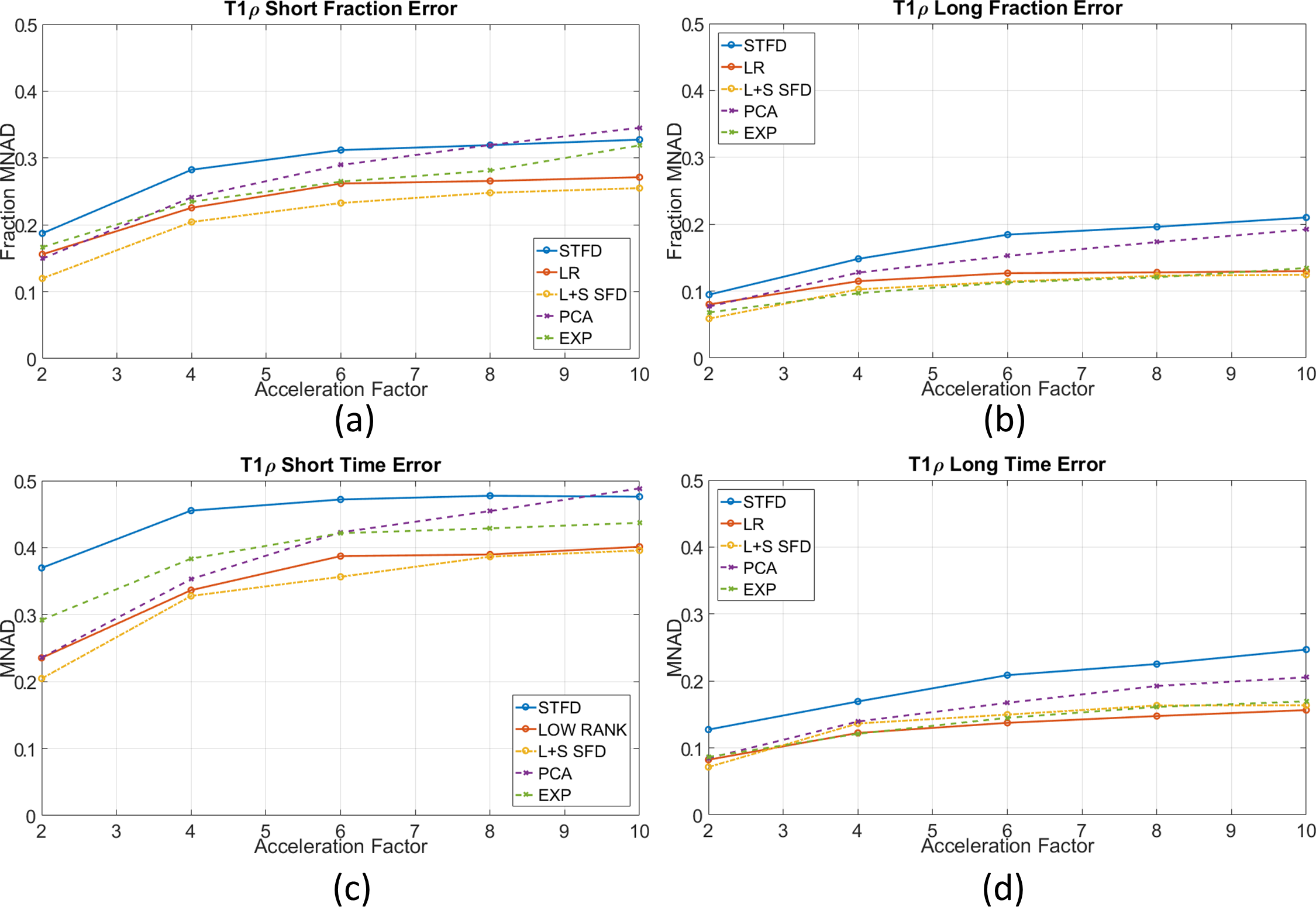
We compare the CS reconstructions and estimated T1ρ relaxation times/fractions with the reference data using normalized root mean square error (nRMSE) and median of the normalized absolute deviation (MNAD) respectively.

Results and Discussion:

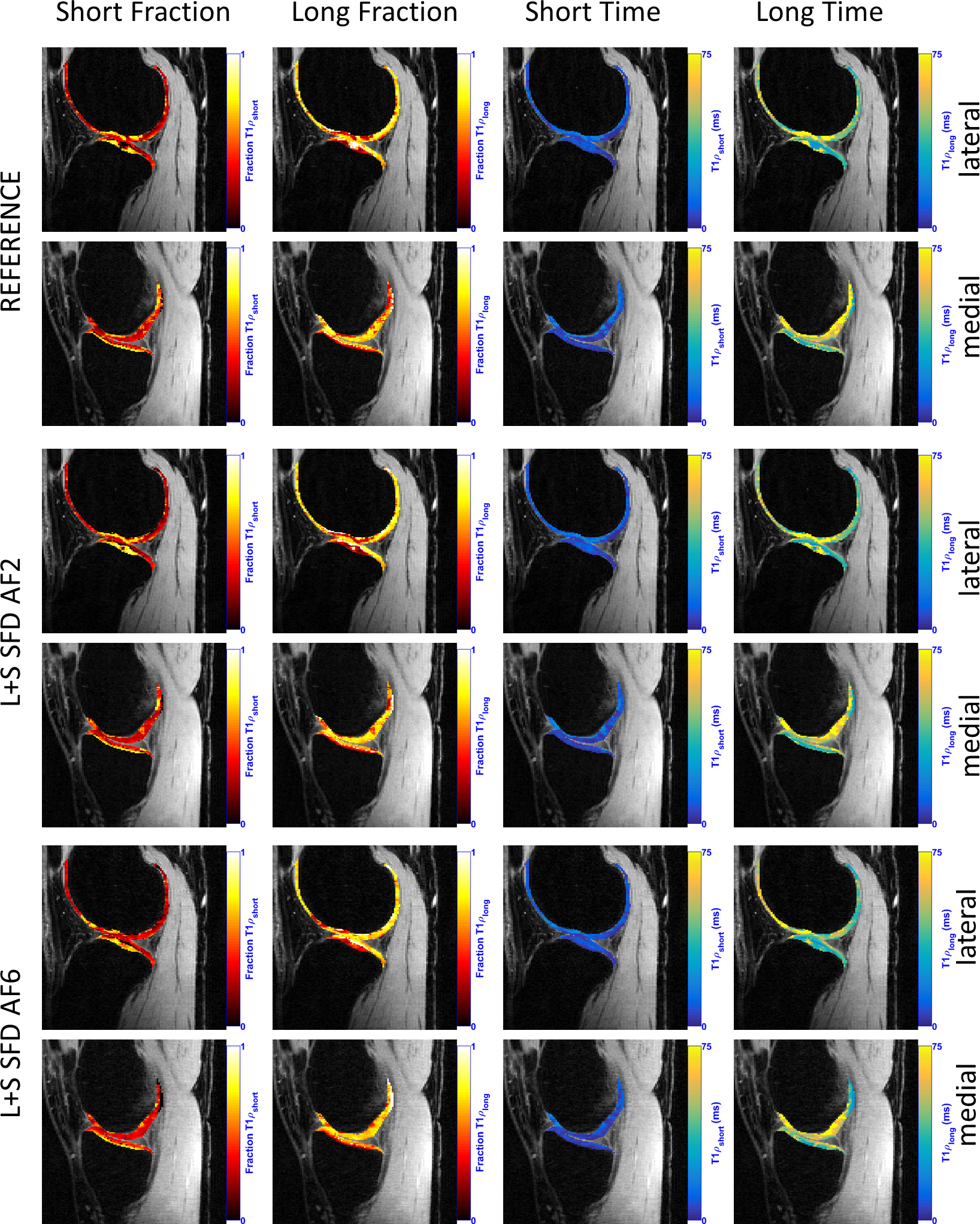
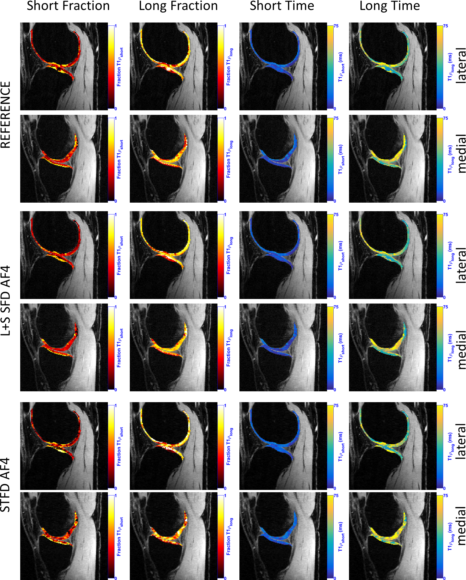
L+S SFD was the best method in terms of biexponential T1ρ mapping of cartilage (Figure 2, visual results on figures 3 and 4), even though it did not present the lowest nRMSE (Figure 1). This is due to the fact that the shape or the error is not considered in the nRMSE, only its size, but it strongly affects mapping results.

The main limitation of STFD is local spatio-temporal correlation, with an usual synthetic look in the images. EXP exploits multicomponent models, highly indicated for this problem, but spatial correlations are not exploited. LR exploits low dimensionality of principal components, similar to PCA, except they are estimated during reconstruction, while fixed in PCA. L+S SFD combines the benefits of LR and sparse models to offer a more natural representation as a superposition of background (global, low rank) and dynamics (local, sparse).

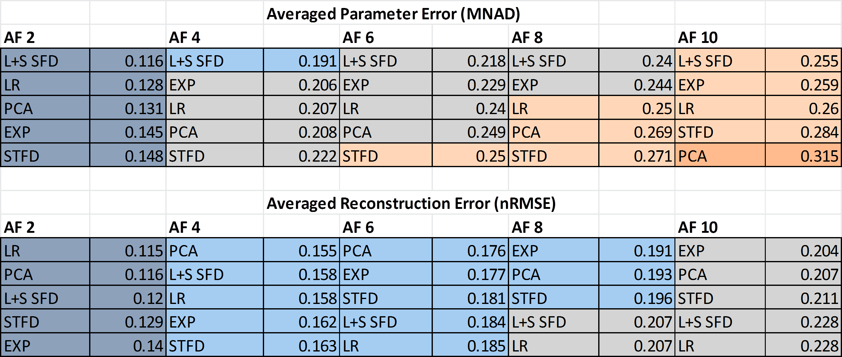
From Table 1, if an error below 0.15 (15%) at MNAD is the target, then AF=2 should be chosen with any method. However, only L+S SFD achieved an averaged MNAD below 0.2 with AF=4. Finally, if an error below 0.25 (25%) at MNAD is the target, then L+S SFD or EXP can be utilized with AF up to 8.

Conclusion:

CS can be used to accelerate biexponential T1ρ mapping of cartilage. L+S model offers best performance among different low-rank and sparse regularization techniques. The CS acceleration will ultimately enable clinically-acceptable acquisition times, which is one of the current limitations of T1ρ mapping.

Acknowledgements

References

[1] A. Sharafi, D. Xia, G. Chang, and R. R. Regatte, “Biexponential T1ρ relaxation mapping of human knee cartilage in vivo at 3T,” NMR Biomed., vol. 30, no. 10, p. e3760, Oct. 2017.

[2] M. Doneva and A. Mertins, “Compressed Sensing in Quantitative MRI,” in MRI: Physics, Image Reconstruction, and Analysis, 2015, pp. 51--71.

[3] M. Uecker, P. Lai, M. J. Murphy, P. Virtue, M. Elad, J. M. Pauly, S. S. Vasanawala, and M. Lustig, “ESPIRiT-an eigenvalue approach to autocalibrating parallel MRI: Where SENSE meets GRAPPA,” Magn. Reson. Med., vol. 71, no. 3, pp. 990–1001, Mar. 2014.

[4] M. Lustig, M. Alley, S. Vasanawala, D. L. Donoho, and J. M. Pauly, “L1 SPIR-iT: autocalibrating parallel imaging compressed sensing,” in Proc. Intl. Soc. Mag. Res. Med, 2009, vol. 17, p. 379.

[5] K. P. Pruessmann, M. Weiger, M. B. Scheidegger, and P. Boesiger, “SENSE: sensitivity encoding for fast MRI.,” Magn. Reson. Med., vol. 42, no. 5, pp. 952–62, Nov. 1999.

[6] H. Jung, J. C. Ye, and E. Y. Kim, “Improved k–t BLAST and k–t SENSE using FOCUSS,” Phys. Med. Biol., vol. 52, no. 11, pp. 3201–3226, Jun. 2007.

[7] M. Elad, P. Milanfar, and R. Rubinstein, “Analysis versus synthesis in signal priors,” Inverse Probl., vol. 23, no. 3, pp. 947–968, Jun. 2007.

[8] D. A. Reiter, P.-C. Lin, K. W. Fishbein, and R. G. Spencer, “Multicomponent T2 relaxation analysis in cartilage,” Magn. Reson. Med., vol. 61, no. 4, pp. 803–809, Apr. 2009.

[9] R. Otazo, E. Candès, and D. K. Sodickson, “Low-rank plus sparse matrix decomposition for accelerated dynamic MRI with separation of background and dynamic components,” Magn. Reson. Med., vol. 73, no. 3, pp. 1125–1136, Mar. 2015.

[10] T. Steihaug, “The conjugate gradient method and trust regions in large scale optimization,” SIAM J. Numer. Anal., vol. 20, no. 3, pp. 626–637, Jun. 1983.