Synopsis

In quantitative susceptibility mapping (QSM), constrained dipole inversion is often necessary to overcome the ill-posedness of the underlying dipole deconvolution problem. Existing methods achieve this by the use of spatial regularization. In this work, we propose a novel "kernel+sparse" model for constrained dipole inversion. In this model, the kernel term absorbs the prior information by representing the susceptibility as a function of prior features while the sparse term accounts for the localized novel features. The proposed method has been evaluated using both simulated and in vivo data, producing impressive results. This method may prove to be useful for many QSM studies.

Introduction

Method

"Kernel+Sparse" Susceptibility Model

The proposed model decomposes the susceptibility distribution $$$\chi$$$ into two terms:$$\hspace{16em}\chi(\boldsymbol{x}_n)=\sum_{i=1}^N\alpha_{i}k(i,n)+\tilde{\chi}(\boldsymbol{x}_n),\hspace{16em}(1)$$where the first component absorbs the prior information and the second one protects the model's ability to represent novel features. The kernel component is motivated by the success of the kernel methods in machine learning². More specifically, we express the susceptibility at each location as a function of a set of features $$$\boldsymbol{f}_n\in\mathbb{R}^p$$$:$$\hspace{16em}\chi(\boldsymbol{x_n})=\Omega(\boldsymbol{f}_n).\hspace{16em}(2)$$The features are extracted from prior images (e.g., anatomical images), which implicitly absorbs prior information directly into the model. However, $$$\Omega(\cdot)$$$ often takes a highly complex form that cannot be accurately linearized in the original feature space^2-3. Inspired by the "kernel trick" in machine learning, $$$\Omega(\cdot)$$$ can be described linearly in a transformed high dimensional feature space spanned by $$$\{\phi(\boldsymbol{f}_n):\boldsymbol{f}_n\in\mathbb{R}^p\}$$$ :$$\hspace{16em}\Omega(\boldsymbol{f}_n)=\omega^T\phi(\boldsymbol{f}_n),\hspace{16em}(3)$$where $$$\phi(\cdot)$$$ is some mapping function and $$$\omega$$$ is a weight vector which also resides in the transformed space⁴:$$\hspace{16em}\omega=\sum_{i=1}^N\alpha_i\phi(\boldsymbol{f}_i).\hspace{16em}(4)$$Hence we obtain the kernel representation for $$$\chi(\boldsymbol{x}_n)$$$ as$$\hspace{16em}\chi(\boldsymbol{x}_n)=\sum_{i=1}^N\alpha_i\phi^T(\boldsymbol{f}_i)\phi(\boldsymbol{f}_n)=\sum_{i=1}^N\alpha_{i}k(i,n),\hspace{16em}(5)$$where $$$k(i,n)=\phi^T(\boldsymbol{f}_i)\phi(\boldsymbol{f}_n)$$$ is the kernel function. In practice, Eq. (5) alone may bias the representation towards the prior information contained in the features. To overcome this potential problem, we introduce a sparse term into Eq. (5) to absorb the localized novel features with the constraint $$$||M(\tilde{\chi}(\boldsymbol{x}_n))||_0≤\epsilon,$$$ where $$$M(\cdot)$$$ is some sparsifying transform.

Dipole Inversion

Specification of the kernel function and features is necessary for the proposed dipole inversion. In this work, we choose the radial Gaussian kernel function$$k(\boldsymbol{f}_i,\boldsymbol{f}_j)=\exp(-\frac{||\boldsymbol{f}_i-\boldsymbol{f}_j||_2^2}{2\sigma^2}).$$ There is considerable flexibility in the choice of features (e.g, image intensities and edge information), which enables the proposed method to absorb a wide range of prior information. The proposed susceptibility model leads to estimation of $$$\chi$$$ from the following optimization problem, $$\hspace{12em}\{\alpha_i^*,\tilde{\chi}^*\}=\arg\min_{\alpha_i,\tilde{\chi}}||D\{\sum_{i=1}^N\alpha_{i}k(i,n)+\tilde{\chi}(\boldsymbol{x}_n)\}-\delta_s||_2^2, s.t. ||M(\tilde{\chi}(\boldsymbol{x}_n))||_0≤\epsilon,\hspace{12em}$$where $$$\delta_s$$$ is the tissue-susceptibility induced field inhomogeneity.

Experiments and Results

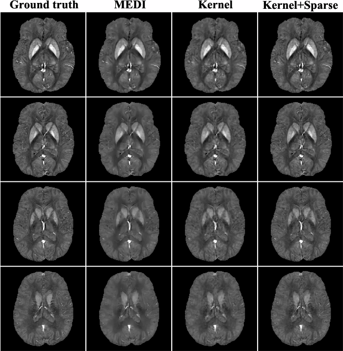
The proposed method has been evaluated using the simulated and in vivo data. The simulated data were generated from the "gold standard" susceptibility distribution in Ref[5] by convolving it with the physical dipole kernel. Figure 1 illustrates the comparison of MEDI¹, kernel-based method without introducing the sparse term and the proposed method. As can be seen, the susceptibility map estimated using MEDI exhibits noticeable blurring effect while the one estimated using the kernel-based model alone also loses some features, although it does recover some fine structures. In contrast the "Kernel+Sparse" model recovers fine structures without the loss of sparse features. The proposed method generates susceptibility estimate with substantially improved accuracy in terms of the relative L₂ norm errors.

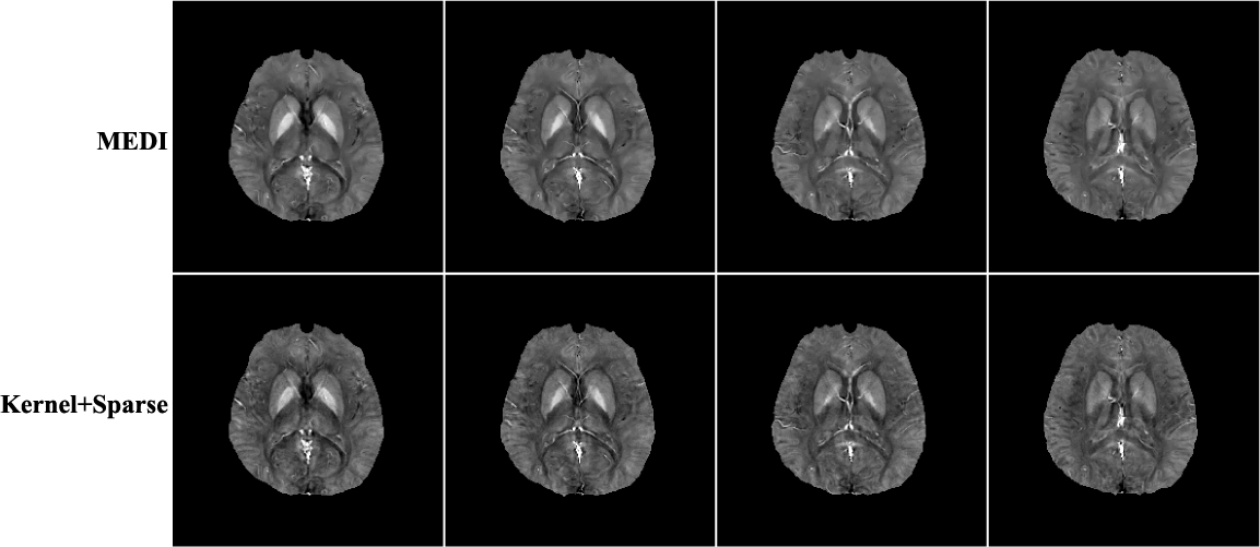
In vivo data were also acquired to demonstrate the capability of the proposed method using a 3D multi-echo GRE acquisition with flow compensation in both slice and readout directions with the following image parameters: 230×230×72 mm³ FOV, 256×256×30 matrix size, 20° flip angle, TR/TE=50/4.55 ms, 3.65 ms echo spacing and 700 Hz BW/pixel. The local magnetic field shift was generated using the Laplacian boundary method⁶. Figure 2 compares the susceptibility map estimated using the proposed method and MEDI. The proposed method outperforms MEDI, capturing more fine structures.

Conclusion

Acknowledgements

References

1. Liu, J., Liu, T., de Rochefort, L., Ledoux, J., Khalidov, I., Chen W, et al. Morphology enabled dipole inversion for quantitative susceptibility mapping using structural consistency between the magnitude image and the susceptibility map. Neuroimage 2012;59:2560-2568.
2. Hofmann T, Schölkopf B, Smola AJ. Kernel methods in machine learning. The annals of statistics 2008:1171-1220.
3. Wang G, Qi J. PET image reconstruction using kernel method. IEEE transactions on medical imaging 2015;34:61-71.
4. Schölkopf B, Herbrich R, Smola A. A generalized representer theorem. In Computational learning theory, Springer Berlin/Heidelberg 2001:416-426.
5. Langkammer C, Schweser F, Shmueli K, Kames C, Li X, et al. Quantitative susceptibility mapping: Report from the 2016 reconstruction challenge. Magn Reson Med 2017 doi:10.1002/mrm.26830.
6. Zhou D, Liu T, Spincemaille P, Wang Y. Background field removal by solving the Laplacian boundary value problem. NMR Biomed 2014;27:312–319.