0193
How should we compare QSM results? A correlation based analysis as an alternative to traditional error metrics1Advanced MRI Section, LFMI, NINDS, National Institutes of Health, Bethesda, MD, United States
Synopsis
During the last QSM Workshop, the results of first “Quantitative Susceptibility Mapping (QSM) Reconstruction Challenge” were presented, which was performed to allow a systematic comparison of various QSM algorithms. One unresolved issue was the fact that the comparison metrics did not properly deal with the effect of smoothing. Here, we propose a comparison method based on pearson correlations, which are calculated over 1D lines throughout the QSM volumes, and show its robustness relative to other metrics under the influence of over-smoothing.
Introduction
In recent years, there have been many numerous methodological improvements in the field of Quantitative Susceptibility Mapping (QSM)1-3. A recent assessment of the current state of the art was performed during the “QSM-Reconstruction-Challenge”, held during the 2016 QSM workshop4. One of the findings of the challenge was that most of the current comparison metrics of QSM performance are not robust in the presence of over-smoothing induced by solving the inverse problem.
During the reconstruction challenge the following metrics were used: root-mean-square-error (RMSE), structural-similarity-index (SSIM), high-frequency-error-norm (HFEN), region-of-interest-based error (ROI). It is well known that some inverse approaches might induce smoothing/blurring on the susceptibility-maps, as algorithms based on compressed-sensing4, or closed-form L2-regularization5. Since, the metrics were not able to properly deal with spatial smoothing, those algorithms gave optimal scores for clearly excessively smooth reconstructions. Also, none of the metrics were successful in optimizing the regularization parameter for a selected algorithm, i.e. total-generalized-variation method4,6.
In this work, we suggest a method based on pearson correlations (r) calculated over 1D lines through the reconstructed QSM volumes, which was also discussed as a future direction in the challenge report4. This approach leads to easily interpretable 2D summary-images of QSM volumes, and the mean r might serve as another metric, while potentially overcoming of comparison with over-smoothed maps.
Methods
We used 3-orientation sampling (COSMOS7) and 12-orientation tensor-map (STI8, ground-truth) solutions that are publicly available4, and calculated susceptibility maps with truncated k-space division (thr=0.2, TKD9), regularized-TKD10 (thr=0.2, TKDreg), closed-form L2 (CF-L25, code provided4). RMSE, HFEN, SSIM and ROI metrics were calculated for each method versus STI. ROI was based on the absolute mean error within a mask provided by the challenge, which was a combination of selected white- and gray-matter regions4. We calculated correlations (r) from multiple lines (left-right, anterior-posterior and inferior-superior) through the QSM reconstructions of the various methods with those of an STI (ground-truth), and reported the volume averaged r values (mean r) to be used as an alternative metric. In addition to comparing the various performance metrics on the different QSM reconstructions, we independently investigated the effects of smoothing. This was done by adding random noise to the STI references, and then applying 3D Gaussian smoothing by using imgaussfilt3 (MATLAB) with increased sigma (standard deviation) values. Finally, we compared all metrics for optimizing the threshold used in TKDreg.Results & Discussion
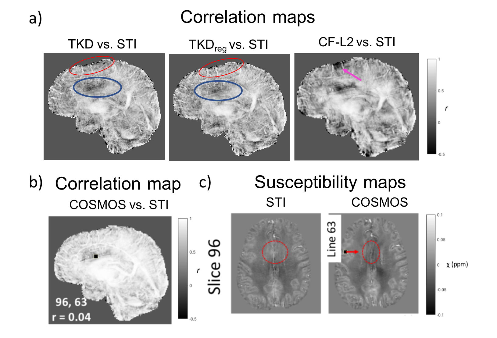
Comparison between methods: We obtained visually similar QSM results within TKD-based methods (Fig. 1), which makes it hard see the differences from exemplary slices, as mostly provided in the reports. Figure 2a,b gives one of three 2D correlation maps derived from 1D-lines (left-right) for each method. From those maps, it is more intuitive to compare different QSM results. We can also extract slice and line information from correlation maps, and check corresponding images, as slice 96 illustrating a region that COSMOS didn’t work well (Fig. 2b,c).
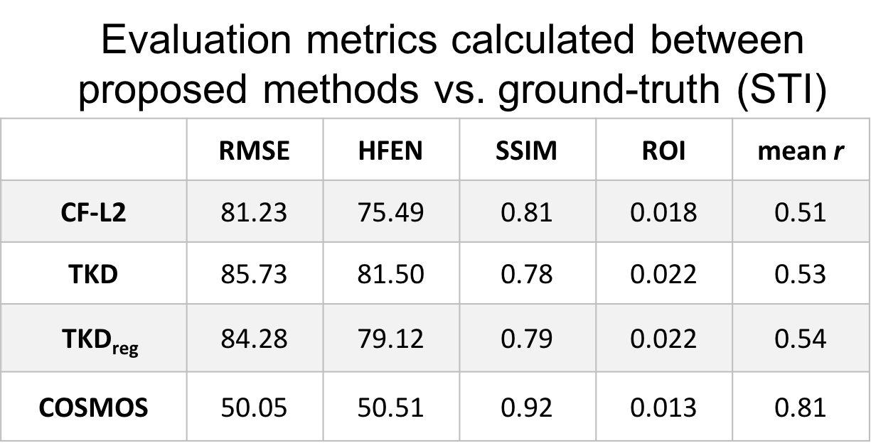
According to RMSEs (Table 1), we can conclude that CF-L2 is the best among others (except COSMOS). However, it is arguable that CF-L2 giving similar/better results for all 4 metrics vs. TKD-based methods (left-most four columns, Table 1), considering that CF-L2 result is overly-smoothed (Fig. 1). As an alternative, mean r values are reported (right-most, Table 1), which gives a more realistic comparison, e.g. CF-L2 gave lowest mean r.
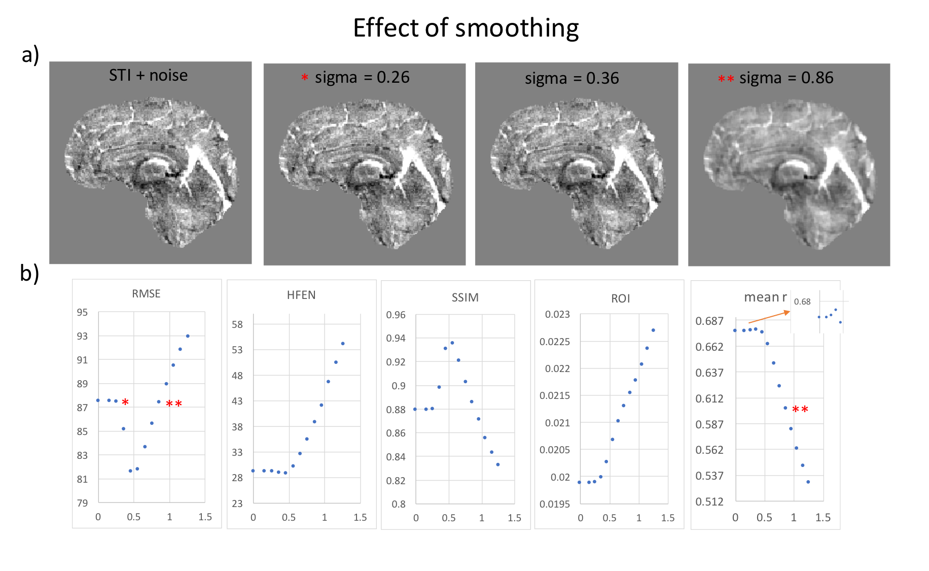
Effect of smoothing: RMSE and SSIM yielded optimum sigma-levels, but achieved similar results between less vs. over-smoothed cases (Fig. 3, compare stars), which clearly doesn’t reflect the reality. ROI gave minimum error without any smoothing on the noisy data. In this case, HFEN and mean r both achieved optimum for sigma values close to 0.4, which potentially helped to reduce the error due to artificially added noise on ground-truth.
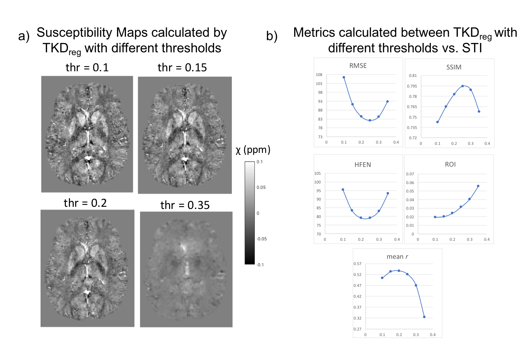
Optimizing TKDreg: ROI approach was not successful to find an optimum threshold for TKDreg. RMSE, SSIM and HFEN metrics found optimum thresholds, yet, achieved similar results between lower vs. maximum threshold (thr=0.35), in which no structural information preserved in the maps (Fig. 4b). All those issues seem to be successfully solved with mean r, by finding an optimum threshold, and making clear distinctions between low and extreme-high cases.
Conclusion
We believe that QSM-researchers might benefit from 2D correlation maps in analyses/reports, which would facilitate visual inspection and quantitative evaluation of performance. As an overall, mean r seemed to be the most robust metric over others considering all scenarios. Specifically, in the case where we wanted to do comparisons between proposed-methods vs. ground-truth, correlation-based metric was the only one which gave lowest score for a smoothing inducing algorithm. We also showed that mean r would -at least- complement others to optimize a parameter for a particular method, especially while trying to avoid over-smoothing.Acknowledgements
This research was supported by the Intramural Research Program of the National Institute of Neurological Disorders and Stroke, National Institutes of Health, Bethesda, MD, USA.References
1. Haacke, E. M. et al. Quantitative susceptibility mapping: current status and future directions. Magn Reson Imaging 33, 1-25 (2015).
2. Wang, Y. & Liu, T. Quantitative susceptibility mapping (QSM): Decoding MRI data for a tissue magnetic biomarker. Magn Reson Med 73, 82-101 (2015).
3. Reichenbach, J. R., Schweser, F., Serres, B. & Deistung, A. Quantitative Susceptibility Mapping: Concepts and Applications. Clin Neuroradiol 25 Suppl 2, 225-230 (2015).
4. Langkammer, C. et al. Quantitative susceptibility mapping: Report from the 2016 reconstruction challenge. Magn Reson Med, doi:10.1002/mrm.26830 (2017). 5 Bilgic, B. et al. Fast image reconstruction with L2-regularization. J Magn Reson Imaging 40, 181-191 (2014).
6. Langkammer, C. et al. Fast quantitative susceptibility mapping using 3D EPI and total generalized variation. Neuroimage 111, 622-630 (2015).
7. Liu, T., Spincemaille, P., de Rochefort, L., Kressler, B. & Wang, Y. Calculation of susceptibility through multiple orientation sampling (COSMOS): a method for conditioning the inverse problem from measured magnetic field map to susceptibility source image in MRI. Magn Reson Med 61, 196-204, doi:10.1002/mrm.21828 (2009).
8. Liu, C. Susceptibility tensor imaging. Magn Reson Med 63, 1471-1477 (2010).
9. Wharton, S., Schafer, A. & Bowtell, R. Susceptibility mapping in the human brain using threshold-based k-space division. Magn Reson Med 63, 1292-1304 (2010).
10. Ozbay, P. S. et al. Effect of respiratory hyperoxic challenge on magnetic susceptibility in human brain assessed by quantitative susceptibility mapping (QSM). NMR Biomed 28, 1688-1696 (2015).
Figures