0191
Vertebral Column Quantitative Susceptibility Mapping using Joint Background Field Removal and Dipole Inversion1Diagnostic and Interventional Radiology, Technical Univeristy of Munich, Munich, Germany, 2Institute of Medical Engineering, Technical University of Munich, Munich, Germany, 3Philips Research Laboratory, Hamburg, Germany, 4Department of Diagnostic and Interventional Neuroradiology, Technical University of Munich, Munich, Germany
Synopsis
Quantitative susceptibility mapping (QSM) with joint background field removal and dipole inversion is applied in the spine of osteoporosis patients and healthy volunteers. Preliminary multi-MR-parametric patient results are compared to low-dose CT scans to investigate the feasibility of QSM to qualitatively and quantitatively detect features of diseased tissues and differentiate positive and negative susceptibility sources in comparison to R2*-mapping.
Introduction/Purpose
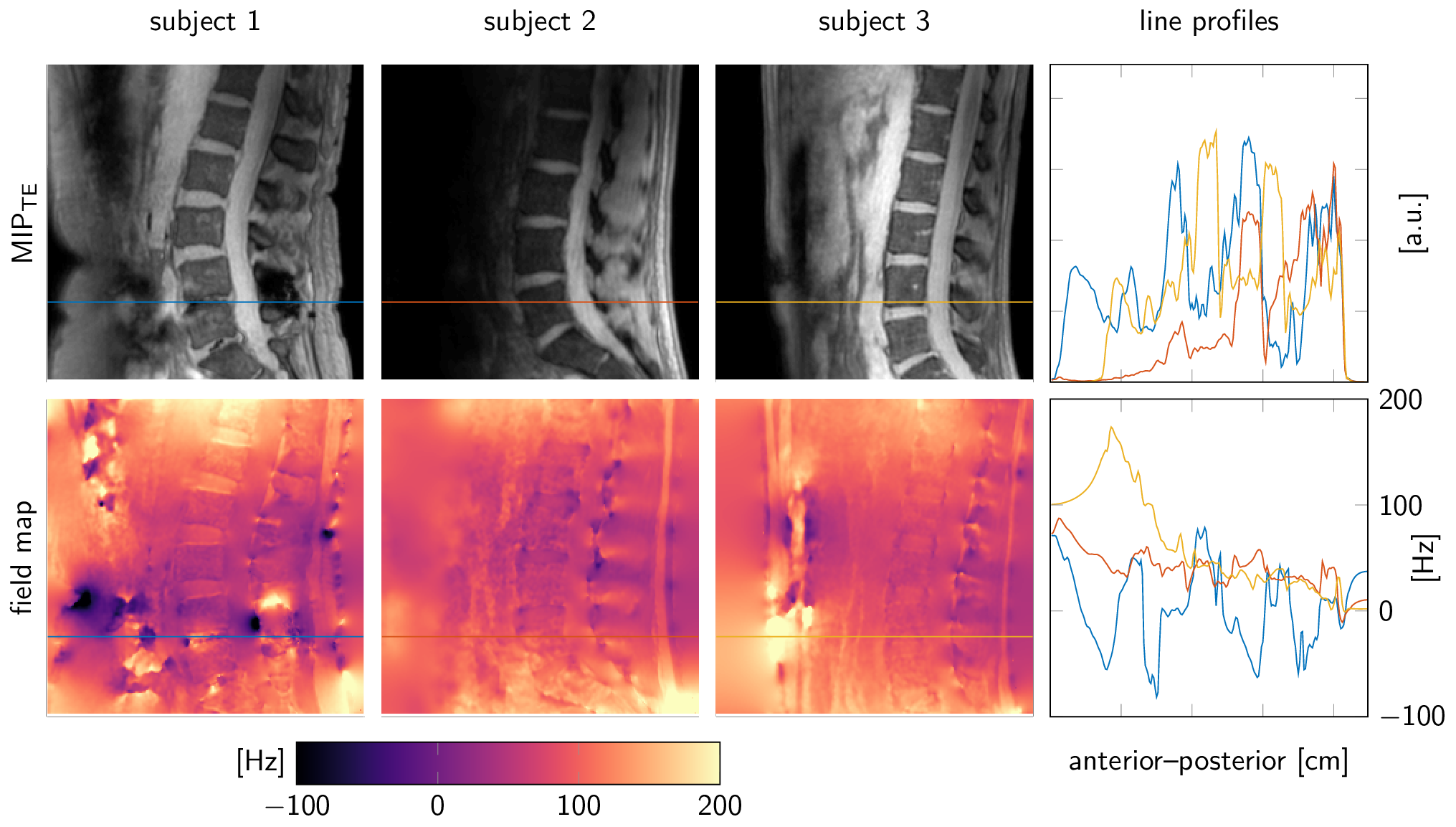
Quantification of magnetic susceptibility effects in the vertebral column has been proposed as a potential approach in order to differentiate calcified structures from disc herniations [1], to assess intervertebral disc health [2] and to measure bone density [3,4]. Quantitative susceptibility mapping (QSM) typically involves three steps: field-mapping, background field removal (BFR) and dipole inversion, which are usually performed sequentially [5]. Popular BFR methods require the definition of a background and a foreground region-of-interest (ROI) based on a masking step [6]. QSM techniques have recently been translated to musculoskeletal tissues in the lower extremities [3,4,7], where volume RF coils are typically employed to encode the signal. Therefore, the entire anatomy lies within the coil coverage and masking background for the BFR step is straightforward. However, MRI of the vertebral column is typically performed using surface coils (typically posterior coil elements) that show a strong signal loss as the distance from the coil increases. Therefore, definition of the background BFR ROI is challenging in the spine due to the inherently inhomogeneous signal profile of the posterior coil (see Figure 1). QSM techniques relying on joint background field removal and dipole inversion do not require the definition of a background ROI [8,9]. The purpose of the present work is to report on the feasibility of vertebral column QSM using a joint background field removal and dipole inversion.Methods
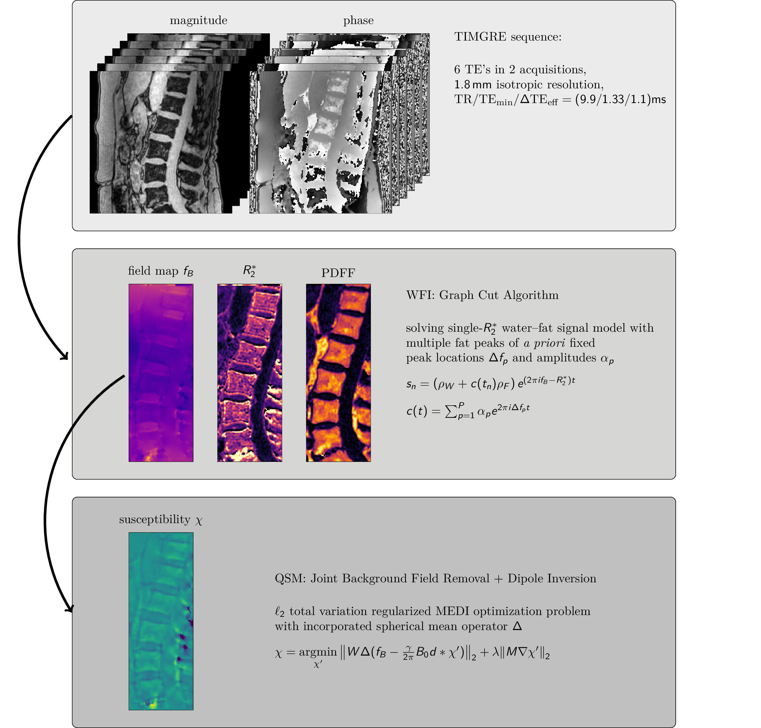
With informed written consent and internal review board ethics approval, a time-interleaved multi-gradient-echo (TIMGRE) sequence [11] with six echoes in two interleaves was applied in six patients (75.8 ± 10years), for whom a low-dose CT was part of the normal radiological care, and three healthy volunteers (27.3 ± 2 years). Sequence parameters involved TR/TEmin/∆TEeff = (9.9/1.33/1.1) ms, FOV = (220 × 220 × 80) mm3 , voxel size = (1.8 mm)3 , flip angle = 3°, scan time = 4:30 min, BWpix = 1504.4 Hz. The TIMGRE sequence allowed to decouple the achievable resolution from the selection of SNR-optimal echo-times for the field mapping [11], which was performed by a graph cut algorithm [12] resulting in unwrapped field maps. The field mapping accounted for the presence of fat, modeled with a 10-peak spectrum specific to bone marrow [13], and a common R2∗-decay for water and fat. For the joint BFR and dipole inversion step the following $$$\ell_2$$$ total-variation regularized optimization problem similar to [5,9] was solved:
$$\chi=\underset{\chi'}{\text{argmin}}\,||W\Delta(f_B-\frac{\gamma}{2\pi}B_0d\ast\chi')||_2+\lambda ||M\nabla\chi'||_2, (1)$$
where fB is the estimated field map, the center frequency $$$\frac{\gamma}{2\pi}B_0$$$, dipole kernel d, magnitude weighting W, and a MEDI-like edge regularization damping M [5]. The first (data-fidelity) term in Equation (1) incorporates the background field removal by exploiting the harmonic properties of the background field. The operator ∆ was implemented as a spherical mean operator with a kernel size of 6 voxels [10]. The regularization parameter λ was heuristically chosen by visual comparison. The resulting susceptibility map χ was not subject to any referencing.
Results
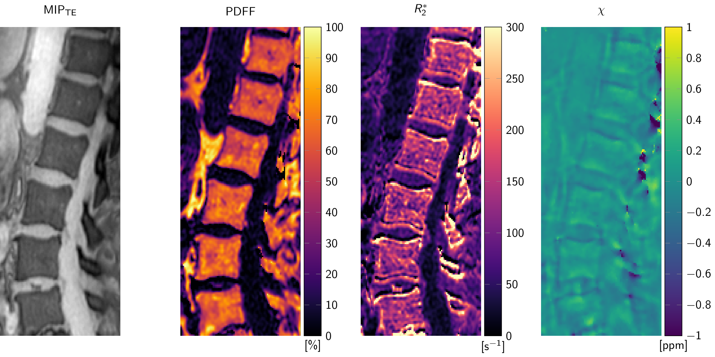
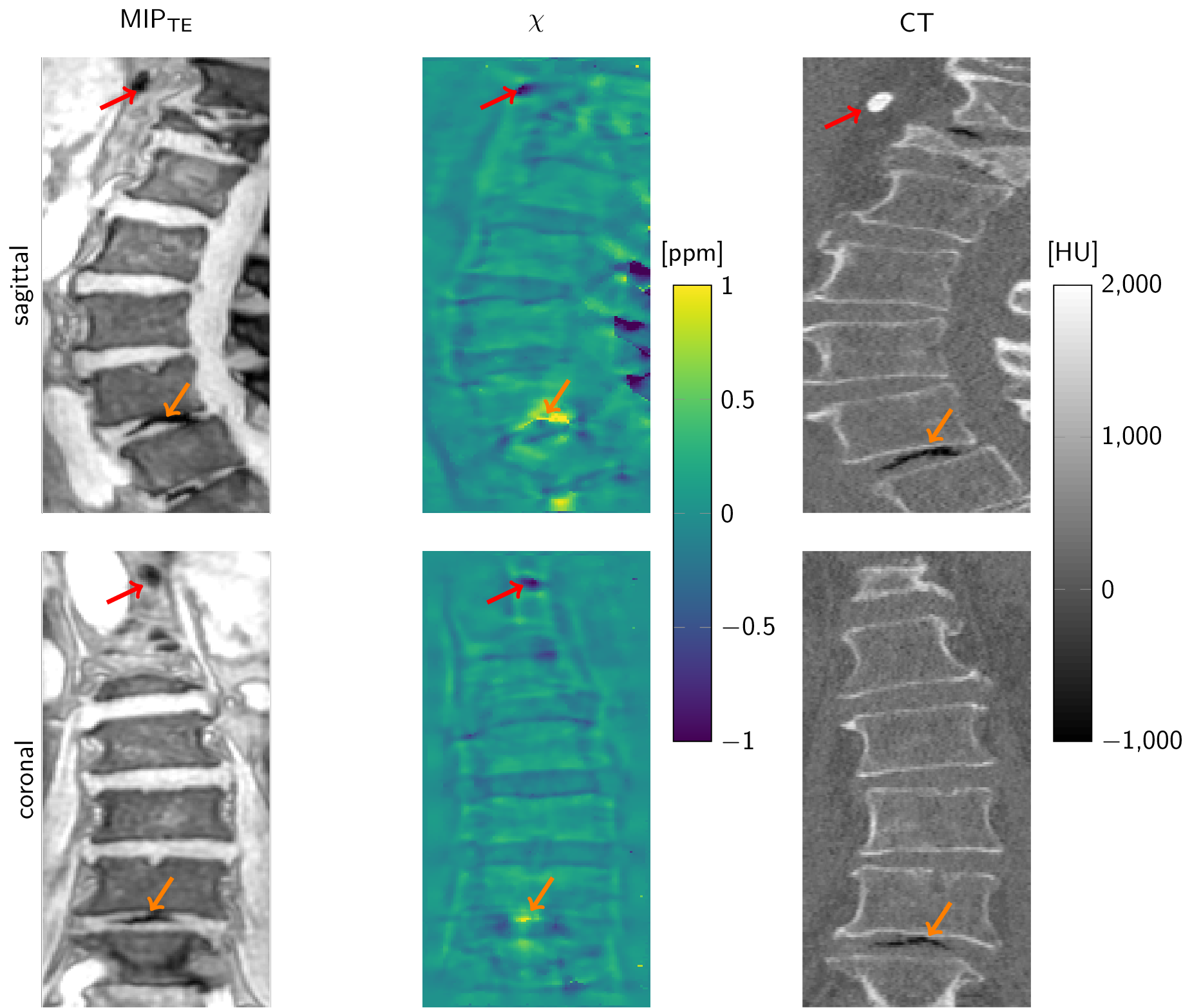
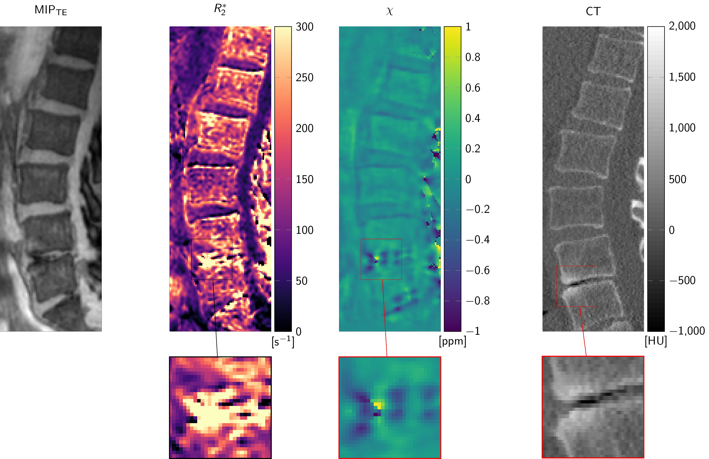
Figure 1 illustrates the differences in signal amplitude problematic for a foreground–background definition. The flowchart in Figure 2 displays the proposed method in performing BFR and dipole inversion jointly to bypass the foreground–background definition. The multi-parametric results of a representative data set from a 76-year-old patient are shown in Figure 3. The QSM maps in Figure 4 show opposite susceptibility of intradiscal air and aortic calcification in a data set of a 81-year-old patient suffering from osteoporosis. In Figure 5 another patient data set (60-year-old) shows susceptibility differences of degenerative changes through bone calcification next to intradiscal air, where both features cannot be detected by the similarly increased intra-voxel dephasing indicated in the R2*-map.
Discussion/Conclusion
QSM results by joint BFR and dipole inversion could consistently be obtained in all data sets. A major challenge is the presence of signal voids inside the thick cortical bone of the spinous and transverse processes. The resulting holes in the field map lead to severe streaking whose mitigation through regularization cause damping of the dynamic range of the susceptibility result. Therefore, quantitative values need to be subject to further optimization. However, qualitative QSM results in the vertebral column could display complementary features of diseased tissue confirmed by CT. The results confirm the theoretical advantage of susceptibility mapping over R2∗-mapping that diamagnetic and paramagnetic susceptibility sources can be differentiated when both similarly result in increased intra-voxel dephasing.Acknowledgements
The present work was supported by the European Research Council (grant agreement No 677661 – Pro- FatMRI) and Philips Healthcare.References
[1] Bender, Y. Y., Diederichs, G., Walter, T. C., Wagner, M., Liebig, T., Rickert, M., Hermann, K., Hamm, B., Makowski, M. R., .., Differentiation of osteophytes and disc herniations in spinal radiculopathy using susceptibility-weighted magnetic resonance imaging, Investigative Radiology, 52(2), 75–80 (2017). http://dx.doi.org/10.1097/rli.0000000000000314
[2] Schick, F., Nagele, T., Lutz, O., Pfeffer, K., & Giehl, J., Magnetic susceptibility in the vertebral column, Journal of Magnetic Resonance, Series B, 103(1), 39–52 (1994). http://dx.doi.org/10.1006/jmrb.1994.1005
[3] Dimov, A. V., Liu, Z., Spincemaille, P., Prince, M. R., Du, J., & Wang, Y., Bone quantitative susceptibility mapping using a chemical species-specific r2* signal model with ultrashort and conventional echo data, Mag- netic Resonance in Medicine, nil(nil), (2017). http://dx.doi.org/10.1002/mrm.26648
[4] Diefenbach et al., Simultaneous R2* and Quantitative Susceptibility Mapping of Trabecularized Yellow Bone Marrow: Initial Results in the Calcaneus, Proc. ISMRM 2017, #850
[5] Wang, Y., & Liu, T., Quantitative suscepti- bility mapping (qsm): decoding mri data for a tissue magnetic biomarker, Magnetic Resonance in Medicine, 73(1), 82–101 (2014). http://dx.doi.org/10.1002/mrm.25358
[6] Schweser, F., Robinson, S. D., Rochefort, L. d., Li, W., & Bredies, K., An illustrated comparison of processing methods for phase mri and qsm: removal of background field contributions from sources outside the region of interest, NMR in Biomedicine, 30(4), 3604 (2016). http://dx.doi.org/10.1002/nbm.3604
[7] Wei, H., Dibb, R., Decker, K., Wang, N., Zhang, Y., Zong, X., Lin, W., Nissman, D. B., Liu, C., .., Investigating magnetic susceptibility of human knee joint at 7 tesla, Magnetic Resonance in Medicine, 78(5), 1933–1943 (2017). http://dx.doi.org/10.1002/mrm.26596
[8] Meineke, Quantitative Susceptibility Mapping in Alzheimer’s Disease using Joint background-field removal and segmentation-Enhanced Dipole Inversion, Proc ISMRM 2016, #4051
[9] Sharma, S. D., Hernando, D., Horng, D. E., & Reeder, S. B., Quantitative susceptibility mapping in the abdomen as an imagingbiomarker of hepatic iron overload, Magnetic Resonance in Medicine, 74(3), 673–683 (2014). http://dx.doi.org/10.1002/mrm.25448
[10] Chatnuntawech, I., McDaniel, P., Cauley, S. F., Gagoski, B. A., Langkammer, C., Martin, A., Grant, P. E., Wald, L. L., Setsompop, K., Adalsteinsson, E., Bilgic, B., .., Single-Step Quantitative Susceptibility Mapping With Variational Penalties, NMR in Biomedicine, 30(4), 3570 (2016). http://dx.doi.org/10.1002/nbm.3570
[11] Ruschke, S., Eggers, H., Kooijman, H., Diefen- bach, M. N., Baum, T., Haase, A., Rummeny, E. J., Hu, H. H., Karampinos, D. C., .., Correction of phase errors in quantitative water-fat imaging using a monopolar time-interleaved multi-echo gradient echo sequence, Magnetic Resonance in Medicine, 78(3), 984–996 (2016). http://dx.doi.org/10.1002/mrm.26485
[12] Hernando, D., Kellman, P., Haldar, J. P., & Liang, Z., Robust water/fat separation in the presence of large field inhomogeneities using a graph cut algorithm, Magnetic Resonance in Medicine, 63(1), (2009). http://dx.doi.org/10.1002/mrm.22177
[13] Ren, J., Dimitrov, I., Sherry, A. D., & Malloy, C. R., Composition of adipose tissue and marrow fat in humans by1h nmr at 7 tesla, Journal of Lipid Research, 49(9), 2055–2062 (2008). http://dx.doi.org/10.1194/jlr.d800010-jlr200
Figures