0190
Quantitative susceptibility mapping using deep neural network1Department of Electrical and Computer Engineering, Seoul National University, Seoul, Republic of Korea, 2Department of Radiology, Harvard Medical School, Boston, MA, United States
Synopsis
In this study, we designed a deep neural network that functions as dipole deconvolution in QSM reconstruction. For label data, COSMOS reconstructed QSM maps were used so that the network produces ground truth like COSMOS results without streaking artifacts. The performance of our network was superior to conventional QSM results with lower RMSE for multiple head orientation input data.
Purpose
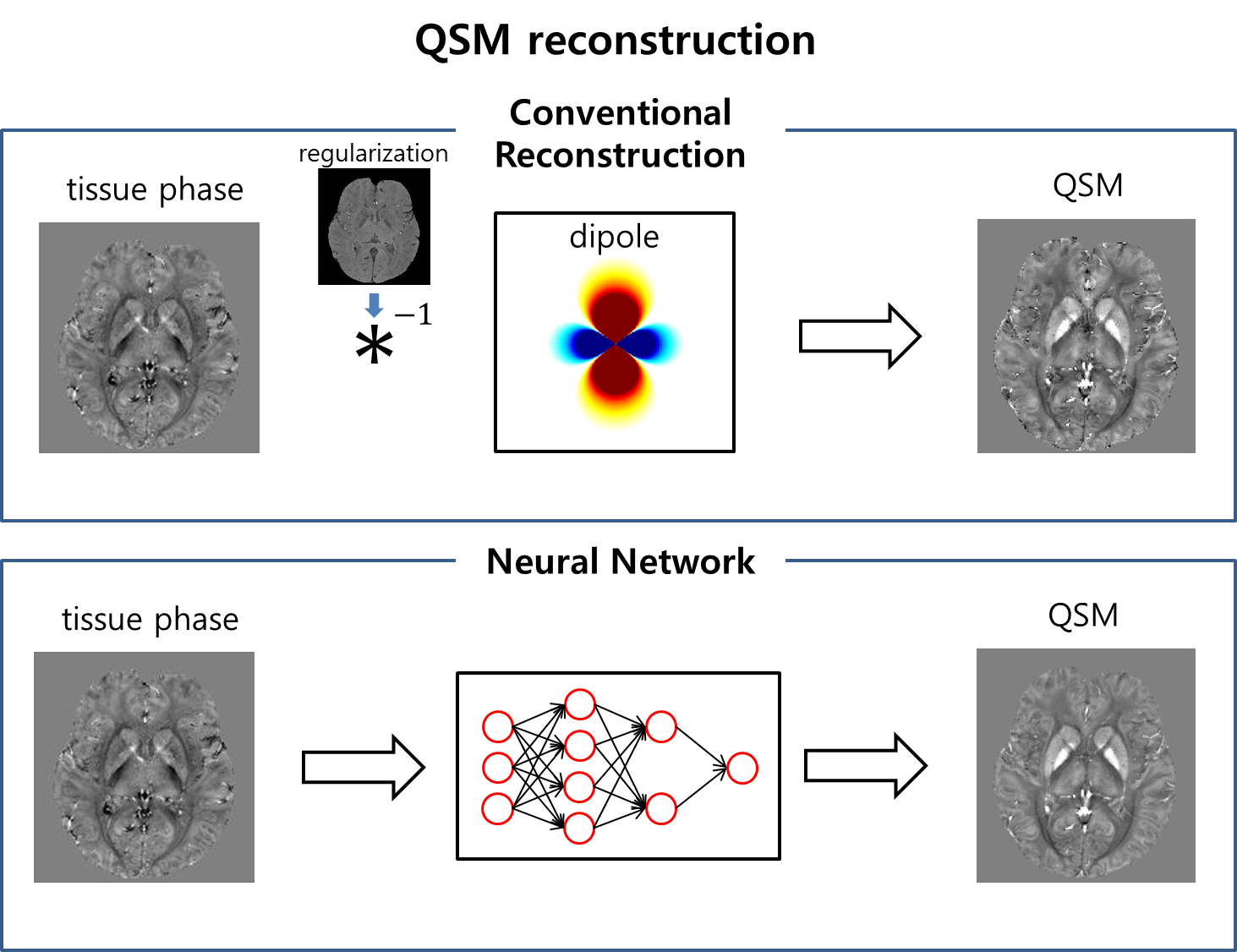
Quantitative susceptibility mapping (QSM) has been proposed as a method to quantify magnetic susceptibility sources. The reconstruction of QSM requires an ill-posed dipole inversion process and, therefore, regularization has been utilized to stabilize the result. The reconstructed images, however, may have unwanted errors because of the regularization imposed during the reconstruction. One solution is acquiring input data in multiple orientations relative to B0 in order to fill out missing information in reconstruction. This approach, which is named COSMOS has successfully generated high-quality QSM results [1] and can be considered as a ground truth when ignoring signal anisotropies in white matter [2,3]. However, it cannot be applied as a routine scan because it requires at least three different head orientation data. In this study, we developed a deep neural network for QSM reconstruction which used COSMOS results for the training to generate COSMOS-quality QSM results (Figure 1).Methods
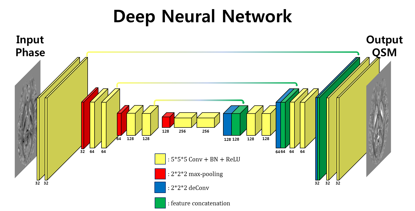
[Deep neural network] QSM reconstruction takes a 3D local field image as an input and generates the same size 3D QSM image. Because the input and the output shares similar structures, feature contracting U-net, which was proposed for biomedical image segmentation [4], was used as a neural network structure. Figure 2 shows the architecture of the proposed network. Since the dipole deconvolution is a 3D process, the U-net structure was modified from 2D to 3D to take 3D inputs and to generate 3D outputs.
[Training] We used multiple orientation local field maps (i.e. a frequency map after removing the background field) as input and COSMOS reconstructed QSM maps as the label. Data from three subjects, each with five different head orientations (resolution=1x1x1 mm3), were used for training (two subject datasets) and testing (one subject dataset). The input image was rotated to have the B0 direction along z-axis so that the network is trained in a consistent B0 direction. For the training, 3D patch with 64x64x64 pixels from local field map was used as an input. The number of training patches was 3360. To overcome data deficiency, we augmented data by generating a local field map from the COSMOS-QSM map in an angle (-300 to 300). Total 3360 patches were augmented resulting in 6720 training patches. For a loss function, we used weighted sum of three losses. The first loss was the L2 loss between an input local field map and a local field map generated by the output QSM map through the dipole convolution (i.e. $$$loss1=||f-d*χ||_2$$$where f is input local field, d is dipole kernel, and χ is output). The second and third losses were the gradient difference losses to compare the edges between the label and output. This loss reduced smoothing effects of the L2 loss and helped to preserve the edges. These losses can be formulated as follows:$$loss2 = ||\triangledown\chi|_x-|\triangledown y|_x|^2+||\triangledown\chi|_y-|\triangledown y|_y|^2+||\triangledown\chi|_z-|\triangledown y|_z|^2$$ $$loss3 = ||\triangledown(d*\chi|)_x-|\triangledown y|_x|^2+||\triangledown(d*\chi)|_y-|\triangledown y|_y|^2+||\triangledown(d*\chi)|_z-|\triangledown y|_z|^2$$where y is the label (COSMOS). The total loss was loss = loss1+λ*loss2+λ*loss3 with λ=1000. After training, one test dataset with five different head orientation was applied to the network to generate QSM maps. The result was compared with conventional QSM using MEDI [5]. The RMSE was calculated between the reconstructed QSM maps and COSMOS result. Additionally, the mean values of each orientation results at five ROIs (Globus Pallidus, Putamen, Caudate, Red Nucleus, and Substantia Nigra) were compared to evaluate consistency of the reconstruction. Computation time for each reconstruction was compared.
Results
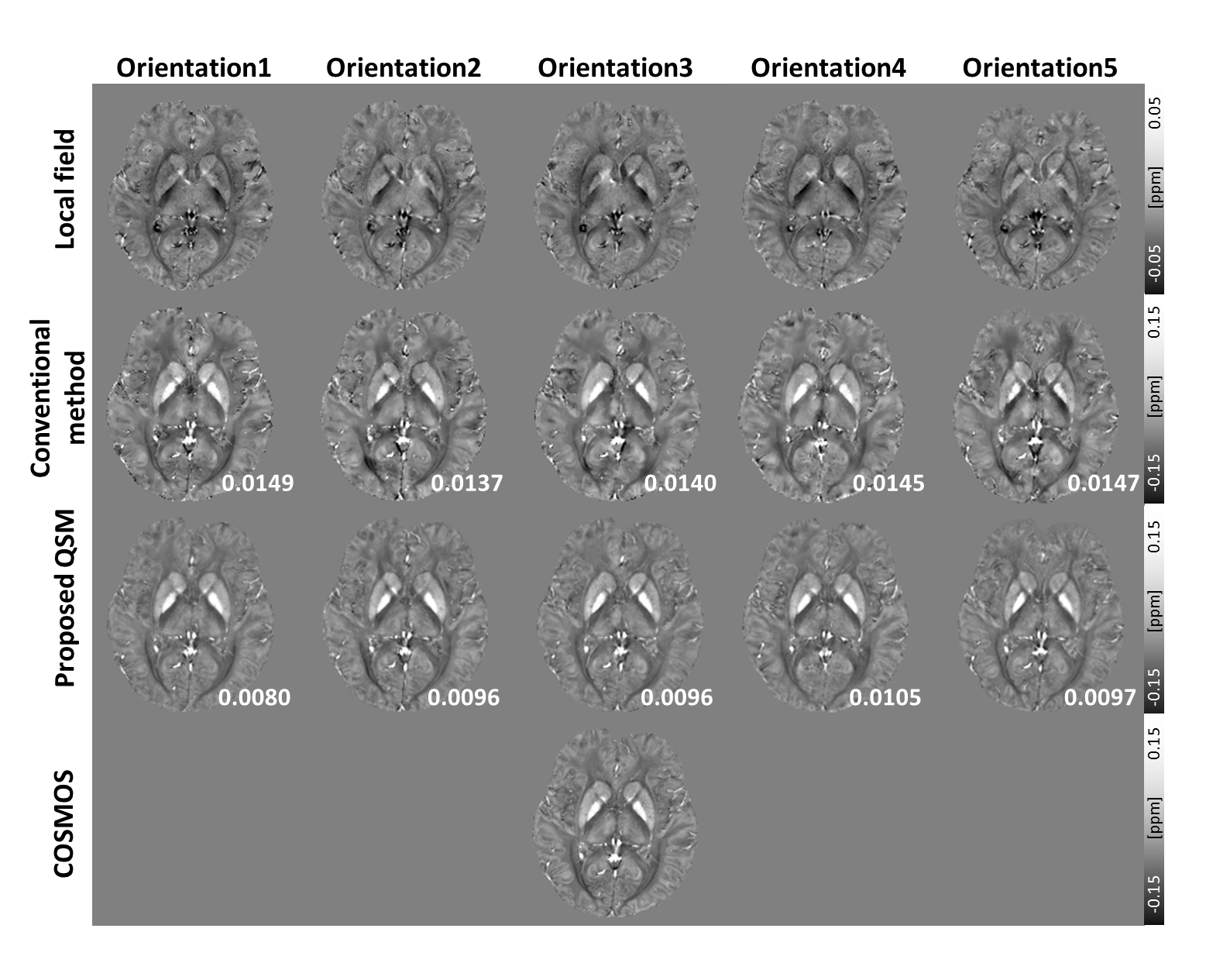
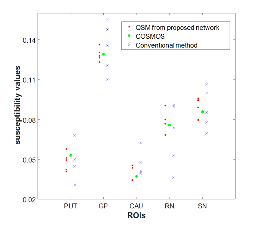
Figure 3 shows the input local field maps of five different head orientations, QSM maps from conventional reconstruction, our neural net reconstruction, and COSMOS reconstruction. Overall, the neural net results reveal great similarity to the ground truth (i.e. COSMOS map), showing less variation across the head orientations. The RMSE error confirms this observation (RMSE: 0.0095 ± 0.0009 in neural net; 0.0144 ± 0.0005 in conventional). Also, the ROI analysis indicates high consistency of the results in our method compared to those from conventional QSM (Figure 4). Another advantage of our neural net is computational time. The neural net generates result within 10 seconds which is close to real-time processing. On the other hand, the conventional reconstruction takes about 5 minutes.
Discussion and Conclusion
In this work, we constructed a deep neural net for dipole deconvolution of QSM reconstruction. The results showed low residuals and the maps were consistent with multiple orientation inputs. On the other hand, the conventional QSM results showed signal variation particularly in white matter, which may originate from anisotropy effectsAcknowledgements
This research was supported by the Brain Research Program through the National Research Foundation of Korea(NRF) funded by the Ministry of Science, ICT & Future Planning (NRF-2017M3C7A1047864).References
[1] Liu T, Spincemaille P, de Rochefort L, Kressler B, Wang Y. Calculation of susceptibility through multiple orientation sampling (COSMOS): a method for conditioning the inverse problem from measured magnetic field map to susceptibility source image in MRI. Magnetic resonance in medicine 61.1 (2009): 196-204.
[2] Lee, Jongho, et al. "Sensitivity of MRI resonance frequency to the orientation of brain tissue microstructure." Proceedings of the National Academy of Sciences 107.11 (2010): 5130-5135.
[3] Wharton, Samuel, and Richard Bowtell. "Fiber orientation-dependent white matter contrast in gradient echo MRI." Proceedings of the National Academy of Sciences 109.45 (2012): 18559-18564.
[4] Ronneberger O, Fischer P, Brox T. U-net: Convolutional networks for biomedical image segmentation. Medical image computing and computer-assisted intervention – MICCAI 9351 (2015): 234-241.
[5] Liu, Tian, et al. Morphology enabled dipole inversion (MEDI) from a single-angle acquisition: comparison with COSMOS in human brain imaging. Magnetic resonance in medicine 66.3 (2011): 777-783.
Figures