Synopsis

Arterial spin labeling (ASL)-based non-contrast enhanced dynamic MR angiography (NCE-dMRA) can provide not only dynamic flow depiction but also quantitative hemodynamics. According to the indicator dilution theory, we proposed a novel analytical solution for arterial blood flow (aBF) quantification in NCE-dMRA. Compared to the previous truncated singular value decomposition (t-SVD), reliable aBF measures were obtained using the proposed method from both simulation and experimental data. Hemodynamic maps including aBF, arterial blood volume and arterial transit time were successfully generated. Our preliminary patient data suggest that the dynamic flow patterns in conjunction with quantitative hemodynamic may provide complementary information for clinical diagnosis.

Purpose

Theory

Dynamic time series of labeled blood signal $$$S(t)$$$ can be expressed by:

$$S(t)=AIF(t)\otimes(aBF\cdot R(t))$$[1]

where $$$AIF(t)$$$ is arterial input function measured in middle cerebral artery (MCA), and $$$R(t)$$$ is residual function which describes the fraction of contrast that remains in the system after a given time $$$t$$$. $$$R(t)$$$ is a positive, decreasing function with $$$R(0)=1$$$, thus $$$aBF=R'(0)$$$ when setting $$$R'(t)=aBF\cdot R(t)$$$.³ Equation [1] can be expressed in discretized matrix form:

$$\begin{bmatrix}S(t_{0}) \\ S(t_{1}) \\ \vdots \\ S(t_{N-1}) \end{bmatrix}=\Delta TI\begin{bmatrix}AIF(t_{0}) & 0 & \dots & 0 \\AIF(t_{1}) & AIF(t_{0}) & \dots& 0 \\\vdots& \vdots& \ddots & \vdots \\ AIF(t_{N-1}) & AIF(t_{N-2}) & \dots& AIF(t_{0}) \end{bmatrix}\times\begin{bmatrix}R'(t_{0}) \\R'(t_{1}) \\\vdots \\R'(t_{N-1}) \end{bmatrix}$$[2]

where N is the number of dMRA frames, and $$$\Delta TI$$$ is the time interval. $$$R'(t_{i})$$$ is regularized by a monotonicity constraint: $$$ R'(t_{i})\geq R'(t_{i+1})$$$, which equals to $$$ P(t_{i})\geq 0$$$ when substituting $$$R'(t_{i})$$$ by $$$P(t_{i})$$$:

$$\begin{cases}P(t_{i})=R'(t_{i})-R'(t_{i+1}) & 0\leq i \leq N-2\\P(t_{i})=R'(t_{i}) & i=N-1\end{cases}$$[3]

Then Equation [2] can be reformatted as:

$$ \begin{bmatrix}\Delta S(t_{0}) \\ \Delta S(t_{1}) \\ \vdots \\ \Delta S(t_{N-1}) \end{bmatrix}=\Delta TI\begin{bmatrix}AIF(t_{0})-AIF(t_{1}) & -AIF(t_{1}) & \dots & -AIF(t_{1}) \\AIF(t_{1})-AIF(t_{2}) & AIF(t_{0}) -AIF(t_{2})& \dots& -AIF(t_{2}) \\\vdots& \vdots& \ddots & \vdots \\ AIF(t_{N-1}) & AIF(t_{N-1})+AIF(t_{N-2}) & \dots&\sum_{\tiny 0}^{\tiny N-1} AIF(t_{i}) \end{bmatrix}\times\begin{bmatrix}P(t_{0}) \\P(t_{1}) \\\vdots \\P(t_{N-1}) \end{bmatrix}$$[4]

$$\begin{cases}\Delta S(t_{i})=S(t_{i})-S(t_{i+1}) & 0\leq i \leq N-2\\\Delta S(t_{i})=S(t_{i}) & i=N-1\end{cases}$$[5]

Solving $$$P(t_{i})$$$ can be considered as a least-squares problem with boundary conditions. Delay and dispersion in AIF are corrected by adjusting the boundary conditions of $$$P(t_{i})$$$:$$\begin{cases}P(t_{i})\leq 0 & t_{i} \leq \tau_d\\P(t_i)\geq0 & t_i > \tau_d\\\sum_{\tiny 0}^{\tiny N-1}P(t_i)\geq 0 \end{cases} $$[6]

where $$$\tau_d$$$ is the delay of AIF, which is estimated by the time when $$$S(t)\geq 0.15\cdot max(S(t))$$$. Equation [5] ensures underlying $$$R'(t_i)$$$ to be a positive function, which peaks at $$$\tau_d$$$, and $$$aBF=R'(\tau_d)$$$. Solving $$$P(t_i)$$$ was implemented in Matlab using ‘active-set’ algorithm.

Methods

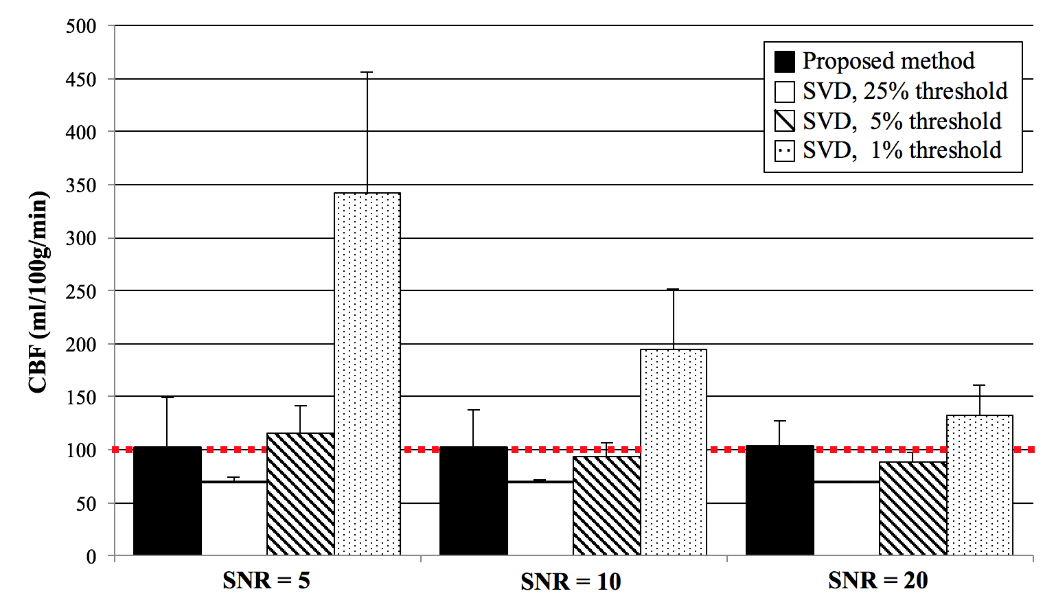
Monte-Carlo simulation was performed to compare the performance of t-SVD and the proposed method at different noise levels. AIF ($$$\tau_d=600ms$$$) and R were simulated by gamma-variate (α=3 and β=150ms) and exponential functions (decay constant=500ms), respectively. S was calculated as convolution between AIF and R assuming $$$aBF=100$$$ml/ml/min and $$$\Delta TI$$$ms. Gaussian noise was added to the time series signal and SNR was defined as average of time series signal divide by the standard deviation of noise. One thousand simulations were performed to calculate $$$aBF$$$ when using the proposed and t-SVD method (SNR=5,10,20).

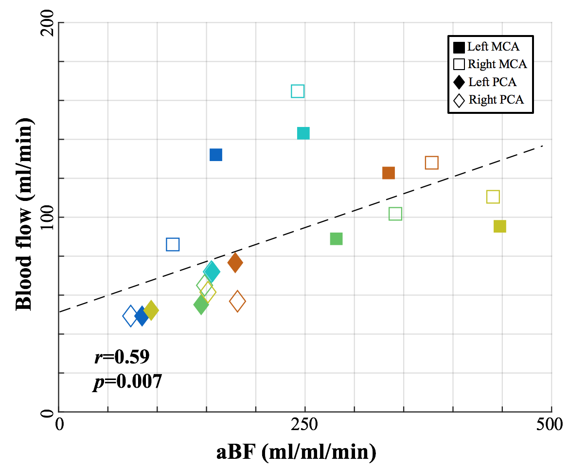
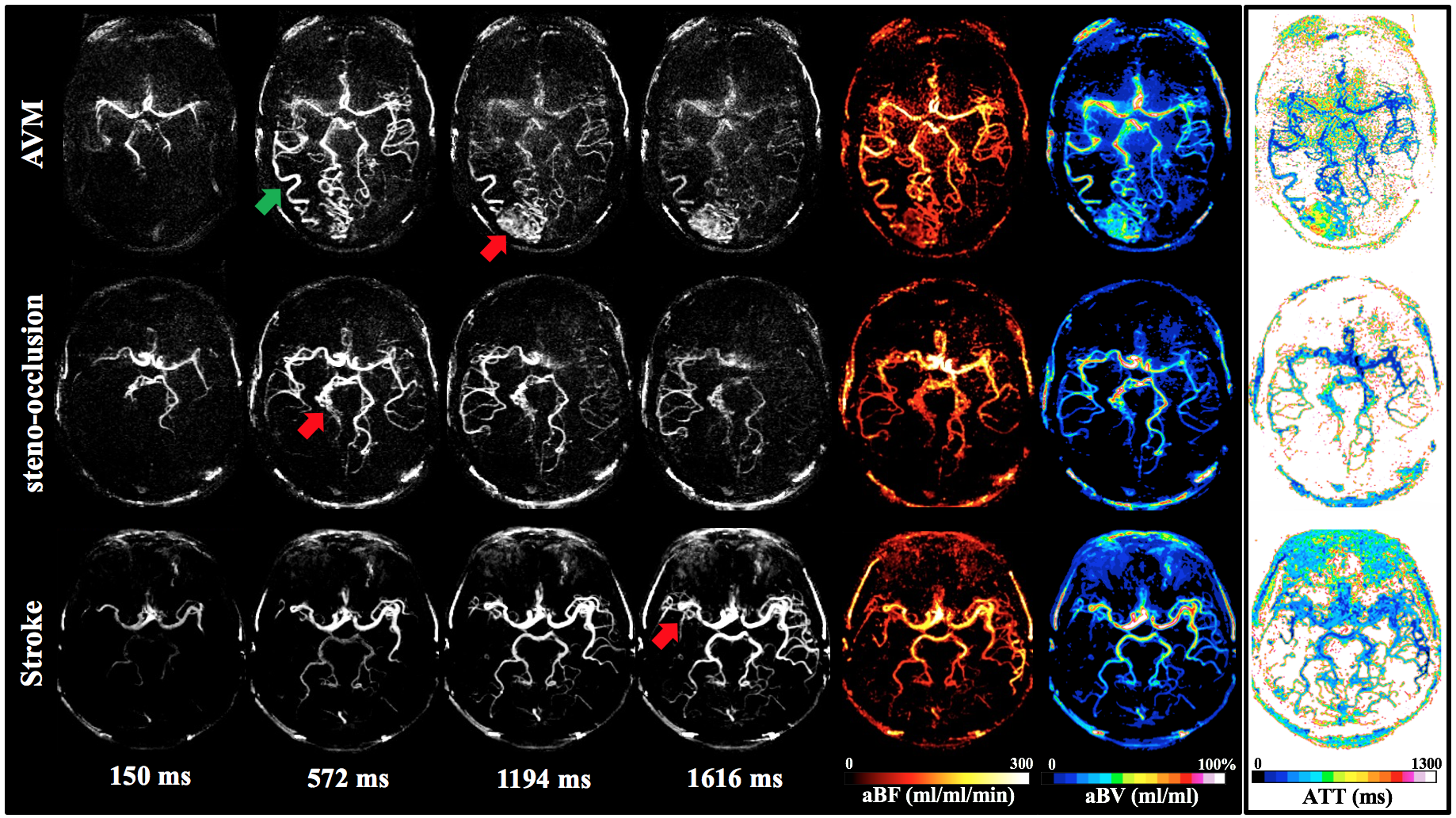
All experiments were performed on a Siemens Tim Trio 3T scanner. Imaging parameters for NCE-dMRA were: voxel size=1x1x1.5mm³, 22 time frames with a temporal resolution of 105.5ms, 32 slices were acquired to cover the circle of Willis and its branches, TA=7.5mins. $$$aBF$$$ was compared with blood flow measured by phase-contrast (PC) MRI (0.5×0.5×5mm³, VENC=80cm/s) at both sides of MCA and posterior cerebral artery (PCA) in five healthy subjects (1M, age=24±2yrs). Hemodynamic parametric maps were generated from three patients with arteriovenous malformation (AVM) (M, age=33yrs), steno-occlusion (F, age=36yrs) and stroke (M, age=58yrs). $$$aBV$$$ and $$$ATT$$$ were calculated by:

$$aBV=\frac{\int S(t)dt}{\int AIF(t)dt},ATT=\frac{aBV}{aBF} $$[7]

Results

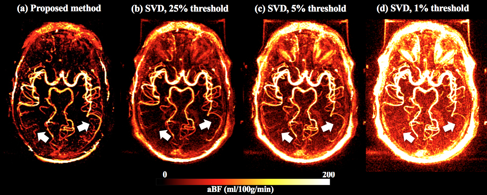
Figure 1 shows the simulated $$$aBF$$$ with the proposed and t-SVD methods. $$$aBF$$$ are highly depended on the threshold in t-SVD method, approximate 5-fold change in $$$aBF$$$ was observed when the threshold was 1% and 25% (SNR=5). In contrast, the proposed method generated reliable $$$aBF$$$ (102.3,101.9,103.4ml/ml/min when SNR=5,10,20). Figure 2 shows $$$aBF$$$ maps from one healthy subject. Significant variation in image intensities was observed in t-SVD method with different thresholds (Fig 2b-d), whereas $$$aBF$$$ map generated by the proposed method shows desirable contrast and better delineation of vessels of all sizes. Significant correlations (P=0.007) between $$$aBF$$$ measured by the proposed method and blood flow measured by PC-MRI were obtained (Figure 3). Figure 4 displays four selected time frames of dMRA images and hemodynamic maps from three patients, providing both dynamic flow patterns and quantitative hemodynamics. Altered hemodynamics through the lesions was observed compared to the contralateral side from the patients.

Conclusion

Acknowledgements

References

[1] Yan L, et al. Unenhanced Dynamic MR Angiography: High Spatial and Temporal Resolution by Using True FISP–based Spin Tagging with Alternating Radiofrequency [J]. Radiology, 2010, 256(1): 270-279.

[2] Murase K, et al, Accuracy of deconvolution analysis based on singular value decomposition for quantification of cerebral blood flow using dynamic susceptibility contrast-enhanced magnetic resonance imaging [J]. Physics in medicine and biology, 2001, 46(12): 3147.

[3] Petersen E T, et al, Model-free arterial spin labeling quantification approach for perfusion MRI [J]. Magnetic Resonance in Medicine, 2006, 55(2): 219-232.