Synopsis

Simultaneous EEG-FMRI data acquisition provides an opportunity for characterization of magnetic field dynamics during imaging, by leveraging the information contained in the EEG induced gradient artefacts. Using a simple effective loop model, we reduce the complex EEG electrode geometry to small effective loops located at off-isocentre positions, which we use to fit first order (linear in space) models of the magnetic field rate of change. From these, estimates of the actual field dynamics, and trajectory/encoding information can be derived at no cost. In this proof-of-principle, we demonstrate estimation of gradient dynamics during a conventional EPI acquisition using simultaneous EEG recordings.

Purpose

Methods

Voltages recorded on the EEG channels are:

$$V_i=-\frac{\partial}{\partial t}{\int}B{\cdot}dA_i+V^{EEG}_{i}$$

where the first term is time-varying flux changes from field dynamics, and the second is scalp potential differences. We henceforth neglect scalp potentials, which are orders of magnitude lower than the gradient-induced voltages⁴, and are averaged over during model fitting.

As the electrodes do not form trivial closed loops, determining the surface over which to integrate is difficult, and induction effects are not attributable to point-locations in space. Here, we propose to model the complex electrode geometries using “effective” conducting loops of infinitesimal area, with offsets from isocentre.

This assumes $$$B=G_x(t)x+G_y(t)y$$$, or that the gradient fields are exactly linear (in space and superposition), ignoring higher order fields and cross-terms. We then simplify the integral as:

$$V_i=-G_{x}'\int x{\cdot}dA_i-G_{y}'{\int}y{\cdot}dA_i$$

$$V_i=-G_{x}'{\cdot}x_i-G_{y}'{\cdot}y_i$$

where $$$G'$$$ denotes the time-derivative. The time-independent integral terms are captured by constant, electrode specific coefficients $$$x_i$$$ and $$$y_i$$$. We can associate these coefficients with the locations of effective loops that integrate to unit area. With calibration, we can determine the subject and setup-specific $$$(x_i,y_i)$$$ for each electrode.

To calibrate, we must assume knowledge of a gradient slew rate, where errors can result in scaling uncertainties in the field estimates. We used a point in the middle of a relatively long gradient slew, to avoid transient effects, and assume nominal gradient values. Our calibration model used gradients at different orientations, to fit:

$$s_i=r_{i}sin(\theta_{gradient}+\phi_i)$$

where $$$r_i=\sqrt{(G'^{2}_{x}+G'^{2}_{y})(x^{2}_{i}+y^{2}_{i})}$$$, $$$\theta_{gradient}=tan^{-1}(G'_y/G'_x)$$$, and $$$\phi_i=tan^{-1}(y_i/x_i)$$$. Once $$$(x_i,y_i)$$$ are calibrated for each electrode, a first order spatial model is used to least-squares fit for $$$G'_x(t)$$$ and $$$G'_y(t)$$$, given $$$V_i(t)$$$. Because the EEG system used samples at 5 kHz, it is not sufficient to fully capture gradient dynamics. Therefore, rather than reconstructing trajectories, we limit our comparison here to a comparison of nominal and measured $$$G'_x$$$ and $$$G'_y$$$ as a proof of principle. The simultaneous EEG-fMRI recordings were performed at 3T, using 64 radial calibration pulses, and tested on a standard EPI acquisition with a readout bandwidth of 2170 Hz/px.

Results

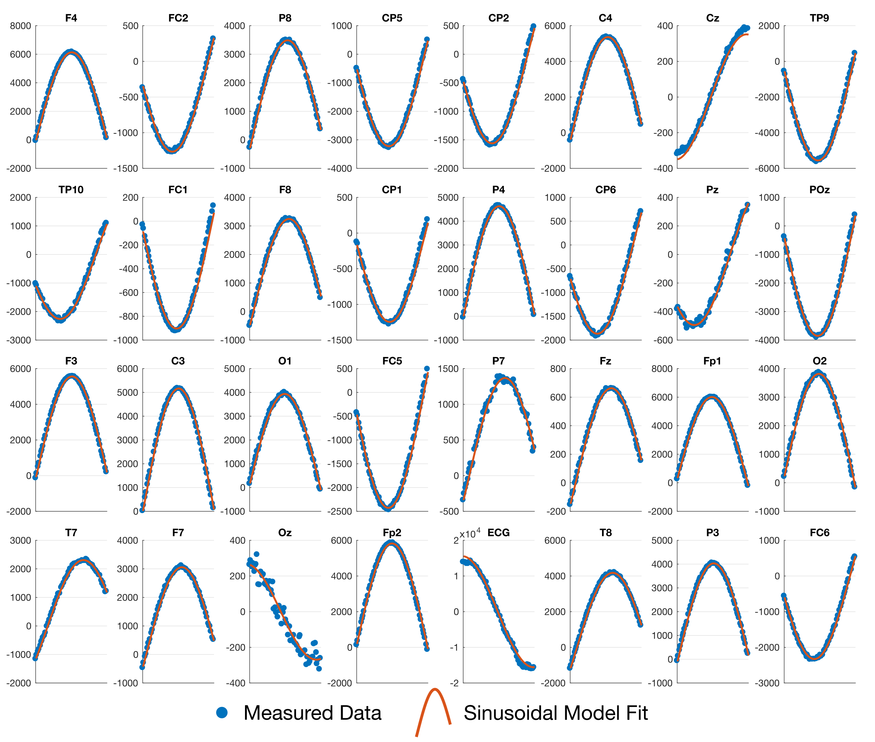
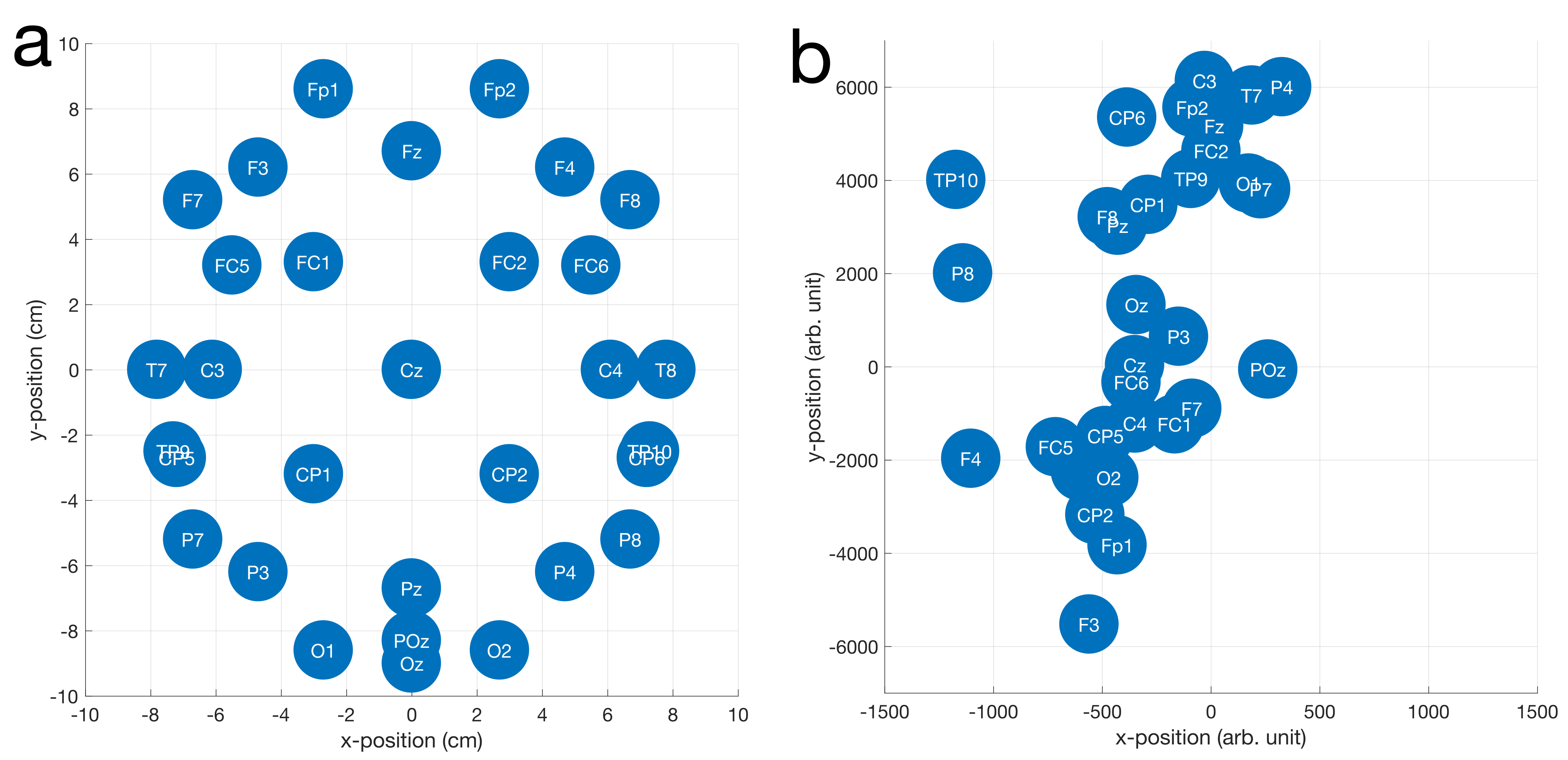
Fig. 1 shows the results of fitting the effective loop models. The excellent correspondence to the model (31/32 electrodes with $$$r^2{\geq}0.99$$$) validates the effective loop approximation. Fig. 2a shows the nominal x-y positions of the electrodes, contrasted with the derived effective loop positions (Fig. 2b). A greater spread of the loop locations in y, compared to x, is possibly due to EEG cabling geometries.

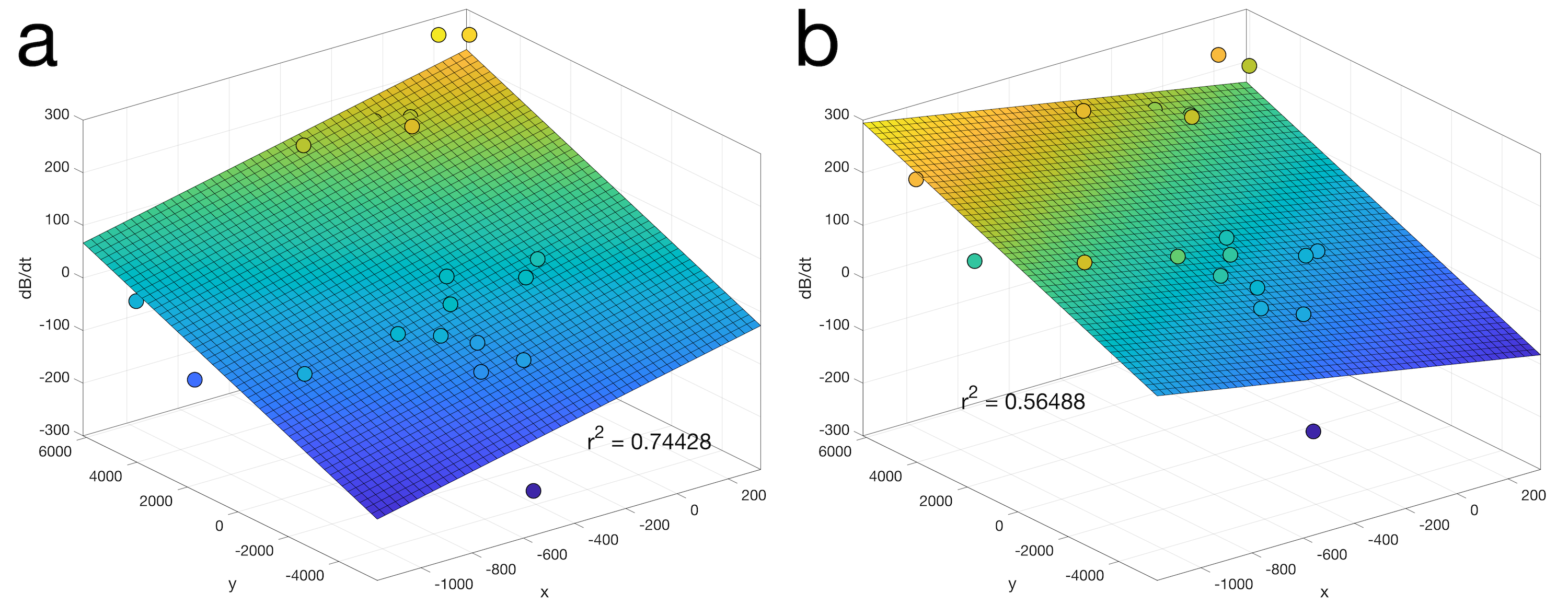
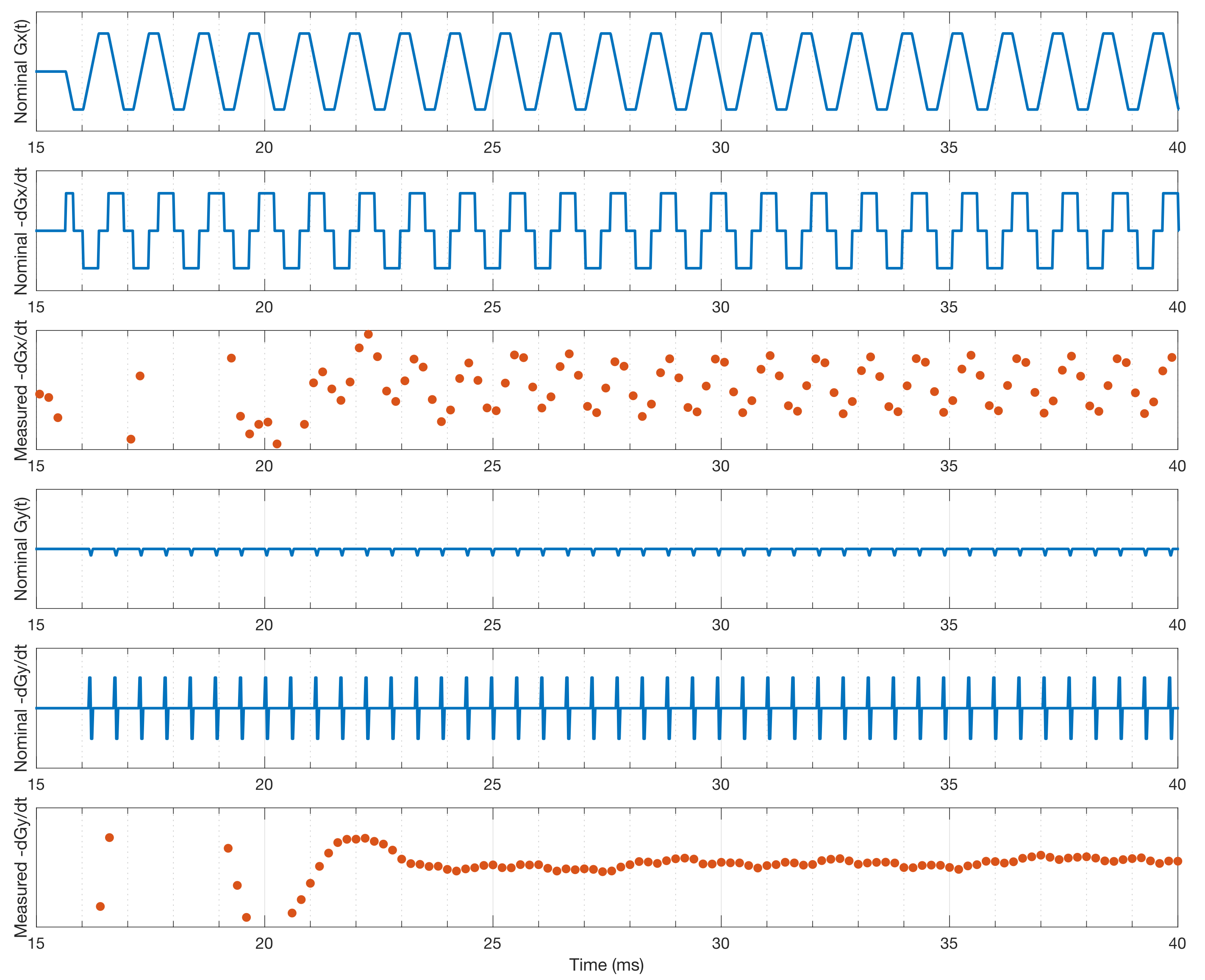
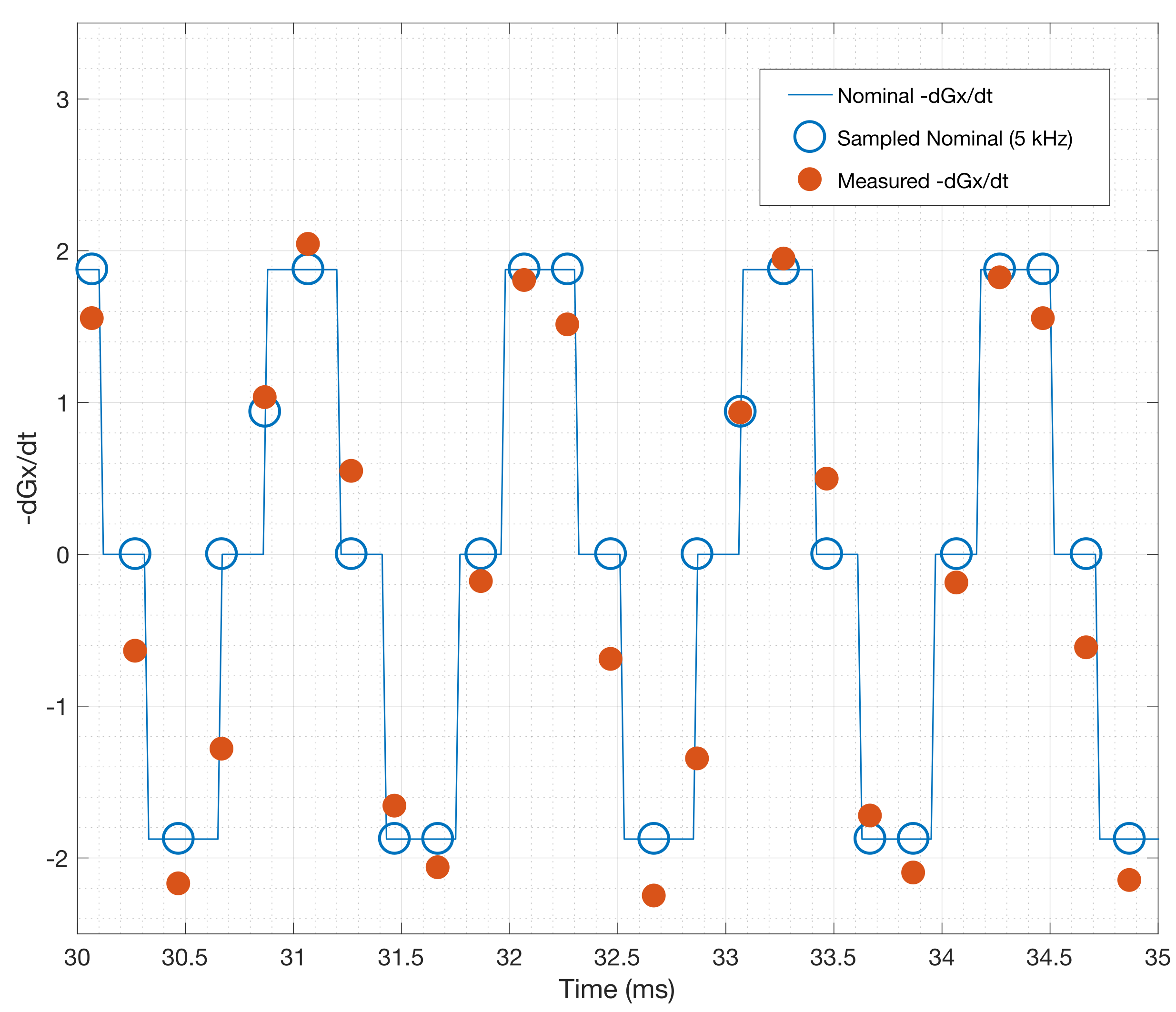
Fig. 3 shows first order fits for the $$$G'_x(t)$$$ and $$$G'_y(t)$$$ coefficients at different points during the EPI readout. Fig. 3a shows the fit during a negative x-gradient slew, and Fig. 3b shows a positive x-slew. The fits range from $$${0.28}{\leq}r^2{\leq}0.96$$$ with a mean of 0.65. Fig. 4 show the nominal $$$G_x$$$, $$$G_y$$$ time-courses during an EPI readout, and associated nominal $$$-G'_x$$$ and $$$-G'_y$$$ time-courses. The EEG-derived $$$-G'_x$$$ and $$$-G'_y$$$ coefficients are plotted for comparison. Fig. 5 shows a zoom in on the $$$-G'_x$$$ estimates, highlighting the intrinsic limits of the 5 kHz EEG sampling. However, the correspondence to the nominal $$$-G'_x$$$ is unmistakable.

Discussion

Acknowledgements

References

1. Barmet, C., Zanche, N. D., & Pruessmann, K. P. (2008). Spatiotemporal magnetic field monitoring for MR. Magnetic Resonance in Medicine, 60(1), 187–197.

2. Vannesjo, S. J., Haeberlin, M., Kasper, L., Pavan, M., Wilm, B. J., Barmet, C., & Pruessmann, K. P. (2013). Gradient system characterization by impulse response measurements with a dynamic field camera. Magnetic Resonance in Medicine, 69(2), 583–593.

3. Deshmane, A., Blaimer, M., Breuer, F., Jakob, P., Duerk, J., Seiberlich, N., & Griswold, M. (2016). Self-calibrated trajectory estimation and signal correction method for robust radial imaging using GRAPPA operator gridding. Magnetic Resonance in Medicine, 75(2), 883–896.

4. Lemieux, L., Allen, P. J., Franconi, F., Symms, M. R., & Fish, D. R. (1997). Recording of EEG during fMRI experiments: Patient safety. Magnetic Resonance in Medicine, 38(6), 943–952.