0175
Improved image quality for long readout imaging using piecewise linear field map model1Bioengineering Department, University of Illinois at Urbana-Champaign, Urbana, IL, United States, 2Beckman Institute, University of Ilinois at Urbana-Champaign, Urban, IL, United States
Synopsis
Trajectories such as spiral or EPI enable fast acquisition compared to spin warp imaging. While a spin warp acquisition has a readout of 2-3 ms, a spiral trajectory readout can be as long as 60 ms. The efficiency of the spiral trajectory comes at a cost of image quality through magnetic field inhomogeneity and T2* decay during long readouts. In this work, a signal model with a piecewise linear field map is used to correct for the magnetic field inhomogeneity effects during long imaging readouts . The proposed method shows the ability to correct for resulting image artifacts.
INTRODUCTION
Spiral or EPI trajectories are SNR efficient and have the advantage of reducing the acquisition time compared to spin warp imaging [1]. While a spin warp acquisition has a readout of 2-3 ms, a spiral readout can be as long as 60 ms. The efficiency of the spiral trajectory comes at a cost of image quality through magnetic field inhomogeneity and T2* decay during long readouts.
Methods for correcting the effects of magnetic field inhomogeneity during the imaging readouts have been previously proposed [2]. Most techniques for magnetic field correction assume that the field map (FM) is piecewise constant. However, intravoxel magnetic field gradients (MFG) induced by magnetic field inhomogeneity exist, resulting in distorted k-space trajectories [3]–[5] which are not modeled by a piecewise constant FM.
In this work, a signal model with a piecewise linear FM is used to correct image artifacts due to intravoxel MFG during long imaging readouts. Corrections for T2* effects have been previously proposed [6]. These corrections are not included here but remain compatible with the proposed framework.
THEORY
The continuous MR signal model is, ignoring the T2* decay [7]:
$$s(t) = \int_{r} f(\mathbf r) \mathrm{e}^{-i \omega (\mathbf r)t} \mathrm{e}^{-i2\pi(\mathbf k(t).\mathbf r)} d \mathbf r$$
The signal model with the piecewise constant FM becomes:
$$s(t) = \sum_{n=0}^{N} f_n \mathrm{e}^{-i \omega_n t} \mathrm{e}^{-i2\pi\mathbf{k}(t)r_n}$$
Including the intravoxel MFG implies that the FM, $$$\omega$$$ is considered as piecewise linear:
$$\omega (r) = \sum_{n=0}^{N} \big ( \omega _n + \mathbf{G}_n \frac{\mathbf{r}-r_n}{\Delta_r} \big ) \phi(\mathbf{r} - r_n)$$
with $$$\phi$$$ the boxcar function, $$$\mathbf{G}$$$ magnetic field gradients.
The MRI signal equation becomes [4], [5]:
$$s(t) = \Delta_r\sum_{n=0}^{N} f_n \mathrm{e}^{-i \omega _n t} \mathrm{e}^{-i2\pi\mathbf{k}(t)r_n} sinc(\mathbf{k}(t) \Delta_r + \frac{\mathbf{G}_nt}{2\pi})$$
METHODS
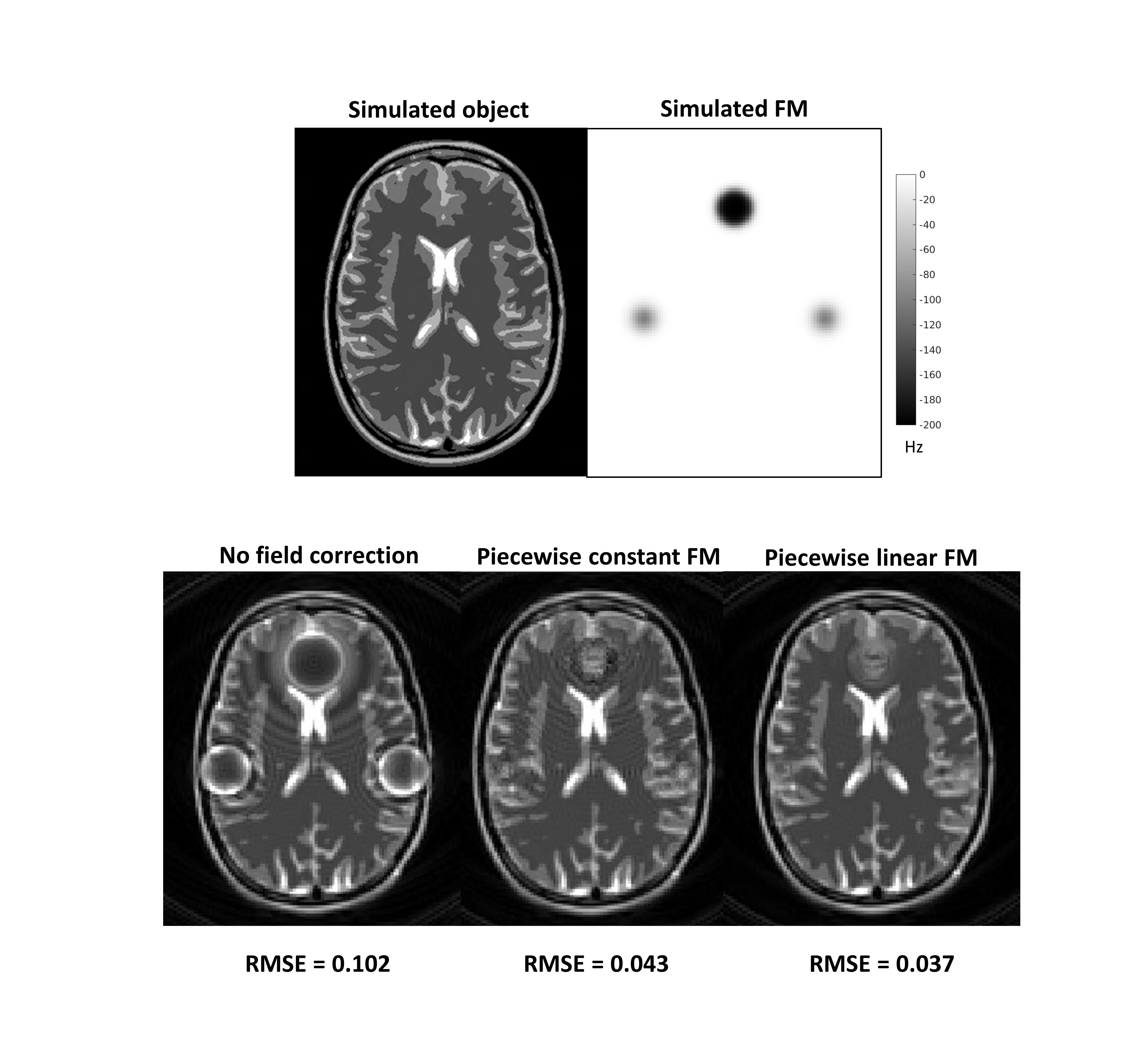
Synthetic k-space data from an analytical brain phantom [8] were generated using the Discrete Fourier Transform (DFT) with the piecewise constant FM model at a resolution 6 times higher than the imaging resolution. A synthetic FM was creating with values ranging up to - 250 Hz/cm, value found in the human brain (Figure 1). A spiral acquisition with a readout duration of 65.2 ms was used for the simulations.
All experiments were conducted on 3 T Magnetom Prisma (Siemens, Erlangen) with a 64-channel head coil. A 2D spin-echo spiral-out sequence was used with: TE=40 ms; TR=200 ms; FOV=24 cm; 40 slices; 1.9x1.9x2 mm3 resolution. Multiple data sets were acquired with different number of shots and readout durations: 1 shot (61.25 ms), 2 shots (30.62 ms), 4 shots (15.31 ms) and 18 shots (3.4 ms).
Images for a sensitivity map and a FM were acquired using a 2D asymmetric spin echo spiral-out sequence with: TE = 15/16.5/22.5 ms; TR = 770 ms; 1.9x1.9x2 mm3; 40 slices; FOV 24 cm; 18 shots. The first echo data were used to estimate coil sensitivity maps while the remaining echoes were used to obtain the FM. Magnetic gradients were obtained using central differences on the estimated field map.
Images were reconstructed using the two signal models combined with the DFT in an iterative image reconstruction approach [9]. To reduce the computational complexity of the fully sampled data, SVD coil compression was used with a rank of 1 as parallel imaging was not the focus of this work.
RESULTS
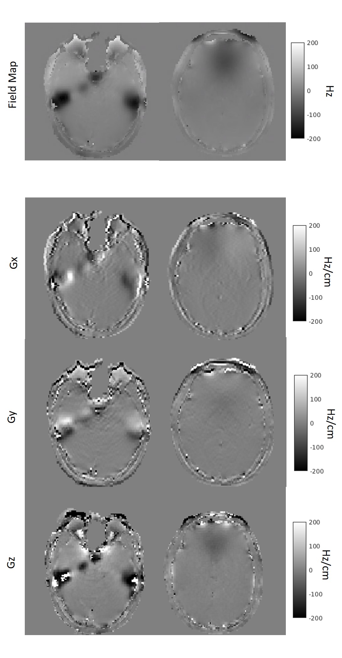
Figure 1 shows the object as well as the FM used for the simulation. Using the piecewise linear FM model improves the quality of the reconstructed image. Figure 2 shows the FM as well as the magnetic field gradient maps for two slices. Those maps were used for reconstructing the images shown in Figure 3. The lower slice experiences MFG as high as -250 Hz/cm, while in the higher slice, the MFG are not as important. For a long readout acquisition such as 1 shot case, using the piecewise linear FM model improved the image quality. For imaging readouts of duration smaller than 15 ms, the piecewise FM linear model does not seem to have an impact on the image.DISCUSSION AND CONCLUSION
For long readout imaging, correction of magnetic field inhomogeneity is necessary to obtain a high image quality, free of magnetic susceptibility artifacts. The impact of intravoxel MFG accumulates during the readout, therefore it is critical to also correct for the intravoxel magnetic field gradients, not just the field map itself. In areas where the magnetic field gradients are strong, images acquired with a long readout imaging can be corrected with the piecewise constant FM model. Some artifacts remain in the images, especially where the magnetic field inhomogeneity gradients are large. In those regions, the distortion of the k-space trajectory from these gradients may have impacted the sampling severely, resulting in an undersampled region.Acknowledgements
This work was supported by the Graduate College at the University of Illinois at Urbana-Champaign.References
[1] L. Kasper et al., “Rapid anatomical brain imaging using spiral acquisition and an expanded signal model,” NeuroImage, Aug. 2017.
[2] B. P. Sutton, D. C. Noll, and J. A. Fessler, “Fast, iterative image reconstruction for MRI in the presence of field inhomogeneities,” IEEE Trans. Med. Imaging, vol. 22, no. 2, pp. 178–188, Feb. 2003.
[3] R. Deichmann, O. Josephs, C. Hutton, D. R. Corfield, and R. Turner, “Compensation of Susceptibility-Induced BOLD Sensitivity Losses in Echo-Planar fMRI Imaging,” NeuroImage, vol. 15, no. 1, pp. 120–135, Jan. 2002.
[4] D. A. Yablonskiy, A. L. Sukstanskii, J. Luo, and X. Wang, “Voxel spread function method for correction of magnetic field inhomogeneity effects in quantitative gradient-echo-based MRI,” Magn. Reson. Med., vol. 70, no. 5, pp. 1283–1292, Nov. 2013.
[5] G.-C. Ngo, C. N. Wong, S. Guo, T. Paine, A. F. Kramer, and B. P. Sutton, “Magnetic susceptibility-induced echo-time shifts: Is there a bias in age-related fMRI studies?,” J. Magn. Reson. Imaging JMRI, vol. 45, no. 1, pp. 207–214, Jan. 2017.
[6] A. Cerjanic, G.-C. Ngo, and B. P. Sutton, “Reducing acquisition time while maintaining spatial resolution wiht extended readouts and R2* modeling,” in ISMRM 25th Annual Meeting and Exhibition, Honolulu, HI, USA, 2017.
[7] Y. Zhuo and B. P. Sutton, “Iterative image reconstruction model including susceptibility gradients combined with Z-shimming gradients in fMRI,” in 2009 Annual International Conference of the IEEE Engineering in Medicine and Biology Society, 2009, pp. 5721–5724.
[8] M. Guerquin-Kern, L. Lejeune, K. P. Pruessmann, and M. Unser, “Realistic analytical phantoms for parallel magnetic resonance imaging,” IEEE Trans. Med. Imaging, vol. 31, no. 3, pp. 626–636, Mar. 2012.
[9] J. A. Fessler, “Penalized weighted least-squares image reconstruction for positron emission tomography,” in 5th IEEE EMBS International Summer School on Biomedical Imaging, 2002., 2002, p. 13.
Figures