0169
GIRF measurement using a combination of triangular and chirp waveform input functions1Philips Research Europe, Hamburg, Germany
Synopsis
Gradient-impulse-response-function (GIRF) measurement is a well-established method for MRI gradient-system characterization. Typical GIRF input-functions are triangles or chirps. For triangles, measurements have to be performed with different pulse lengths to get a continuous frequency spectrum due to blind spots in the spectrum, requiring long scan times. In contrast, the spectrum of the chirp waveform covers a large frequency range without blind spots. However, at low frequencies the chirp fails due to a diverging intensity in its spectrum. We interleaved both waveforms and obtained a continuous gradient modulation transfer function (GMTF) spectrum down to low frequencies in short measurement time.
Purpose:
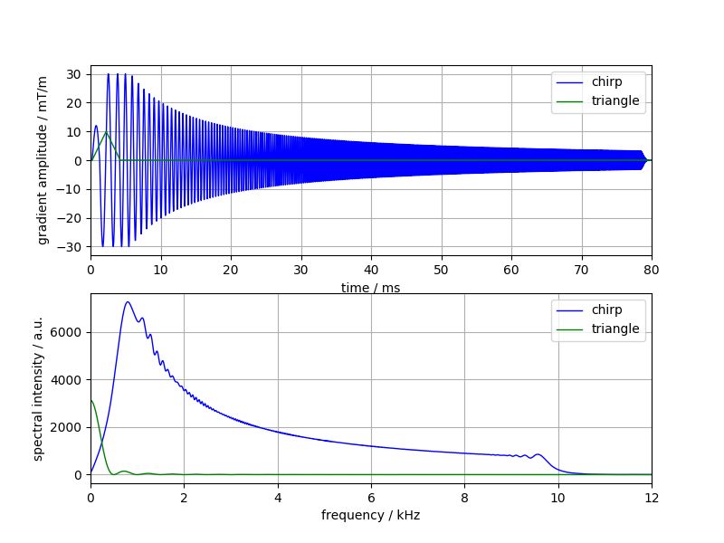
Fast imaging sequences require rapid switching of strong gradient fields during signal readout. These field variations generate eddy currents that lead to substantial deviations from the expected k-space trajectory. Measurement of the gradient impulse response function (GIRF) is a well-established method for characterization of MRI gradient system under the assumption of linear time-invariant behavior. It can be used for characterization of field imperfections, as caused by eddy currents, concomitant fields, and mechanical gradient coil oscillations1 and for the derivation of more accurate k-space trajectories2. Different input functions are used for GIRF measurements like triangles3 or so-called chirps4. For triangles, repeated measurements have to be performed with different triangle pulse lengths to get a continuous frequency spectrum due to blind spots in the triangle spectrum, which is a squared Sinc function (Fig. 1 bottom, green). This approach thus requires long scan times of 1 hour and more5. In contrast, the spectrum of the chirp waveform (Fig. 1 bottom, blue) covers a large frequency range without blind spots and with high spectral density and therefore enables time-efficient measurement of the GIRF in a single scan per gradient axis. However, at low frequencies, its spectral density approaches zero, leading to a diverging intensity in the spectrum of the gradient modulation transfer function (GMTF), i.e. the Fourier transform of the GIRF. To overcome the disadvantages of the individual methods, we interleave both waveforms in a single measurement to obtain a continuous GMTF spectrum down to low frequencies in short measurement time.Methods:
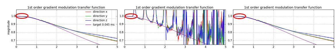
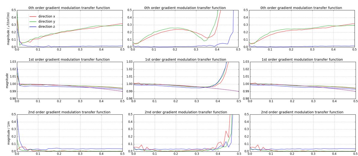
Measurements were performed on a 3T Philips Ingenia system (Philips Healthcare, Best, The Netherlands) with a spherical phantom (diameter: 17cm, standard CuSO4 solution) without additional hardware. We used the method of generating a virtual 1D test probe by thin slice selection6 for all three gradient axes. To probe the spatial variation of the system response, we shifted the positions in selection direction7, so that we acquired signal from three stacks (x-, y-, z-gradient) with four slices each (slice distance 20mm, thickness 1.4mm). The duration of the applied slew-rate limited chirp4 is 80ms and its frequency modulation ranges from 400Hz to 10kHz. The acquisition window is also 80ms, the maximal gradient strength is 30mT/m, and the maximum slew rate is 200mT/m/ms. The triangle shaped gradient, needed for the low frequency characterization, has a duration of 4ms and a maximal gradient strength of 10mT/m. The acquisition window is 80ms as well (Fig. 1, top). The complete measurement time was approx. 3 minutes. The GMTFs of the chirp, of the triangle, and the combination of both3 were calculated in terms of 0th, 1st, and 2nd spatial order along the gradient direction (Figs. 2 and 3, left: chirp, mid: triangle, right: combination).Results:
The GMTF of the measurement using only the chirp waveform shows a well tempered behavior above approx. 100Hz, but is very unreliable below this frequency. In contrast, the GMTF of the triangle can be used for frequencies below 200Hz. A combination of both by a spectral weighted superposition gives a smooth spectrum with good SNR over the frequency range of interest. This can be observed in all spatial orders evaluated.Discussion and Conclusion:
For characterization of the gradient response, we demonstrated that a combination of chirp and triangle shaped test gradients can significantly reduce scan time without losing information frequencies below the lower cutoff frequency of the chirp waveform.Acknowledgements
No acknowledgement found.References
[1] Graedel, N. N. et al. Image reconstruction using the gradient impulse response for trajectory prediction. Proc. Intl. Soc. Mag. Reson. Med. 21, 552 (2013)
[2] Campbell-Washburn, A. E. et al. Real-Time Distortion Correction of Spiral and Echo Planar Images Using the Gradient System Impulse Response Function. Magnetic Resonance in Medicine 75, 2278–2285 (2016)
[3] Vannesjo, S. J. et al. Gradient system characterization by impulse response measurements with a dynamic field camera. Magn. Reson. Med. 69, 583–593 (2013)
[4] Addy, N. O., Wu, H. H. & Nishimura, D. G. Simple method for MR gradient system characterization and k-space trajectory estimation. Magn. Reson. Med. 68, 120–129 (2012)
[5] Vannesjo, S. J. DISS. ETH NO. 21558 (2013)
[6] Duyn, J. H., Yang, Y., Frank, J. A. & van der Veen, J. W. Simple Correction Method for k-Space Trajectory Deviations in MRI. J. Magn. Reson. 132, 150–153 (1998)
[7] Gurney, J. M. et al. A simple method for measuring Bo eddy currents. Proc. Intl. Soc. Mag. Reson. Med.13 (2005)
Figures